Download
1 / 13
130 likes | 236 Views
Short Time Calculations of Rate Constants for Reactions. With Long-lived Intermediates. Maytal Caspary , Lihu Berman, Uri Peskin Department of Chemistry and The Lise Meitner Center for Computational Quantum Chemistry, Technion – Israel Institute of Technology, Haifa 32000, Israel.

E N D
Short Time Calculations of Rate Constants for Reactions With Long-lived Intermediates Maytal Caspary, Lihu Berman, Uri PeskinDepartment of Chemistry and The Lise Meitner Center for Computational Quantum Chemistry, Technion – Israel Institute of Technology, Haifa 32000, Israel M. Caspary, L. Berman, U. Peskin, Chem. Phys. Lett. 369 (2003) 232. M. Caspary, L. Berman, U. Peskin, Isr. J. Chem. 42 (2002) 237.
Defining the problem Consider a case where there is an intermediate state in a reaction that is associated with a long-lived resonance state. Example:
W.H. Miller et. al introduced a powerful expression for the rate constant calculation: The practical form is:
The Solution The rate can be calculated at any one of the barriers: The expressions for the rate constant can be represented as infinite time limits:
The NEW method Defining a time-dependent weighted average of the two integrals: The rate can be written exactly as:
Rewriting the time integrals After substitution: If the asymptotic limit is obtained at a finite time
Lets assume that at the dynamics is dominated by the decay of the resonance: The flux correlation functions decay asymptotically in time and the convergence of their time integrals can be accordingly slow: In the case of a resonance dominating the dynamics at any ,
Result:The Flux Averaging Method A “working equation” for the rate constant which is formally exact:
Numerical Examples: One-dimensional symmetric potential barriers The rate constant for the double barrier potential shown above was calculated in three different ways: The new expression converges to the asymptotic value much faster than each one of the time integrals whose convergence is limited by the resonance decay time.
One-dimensional asymmetric potential barriers The method is applicable for the more common asymmetrical case. The contribution of each correlation function to the weighted average is non symmetric.
Multiple resonance states The method can be generalized for situations in which a number of resonance states contribute to the reaction rate, and the decay process is accompanied by an internal dynamics within the quasi-bound system. asymmetric potential barriers
Conclusions: • In this work we propose a new expression for the calculation of the thermal rate constant, which circumvents the problem of long time dynamics due to resonance states. • By averaging (“on the fly”) different time-integrals over flux-flux correlation functions, a formally exact expression is obtained, which is shown to converge within the time scale of the direct dynamics, even when a long-lived resonance state is populated. • In addition, a generalized flux averaging method is proposed for cases where the dynamics involve more than a single resonance state. • Numerical examples were given in order to demonstrate the computational efficiency.