Download

1 / 50
530 likes | 590 Views
3. CHAPTER. Demand and Supply. After studying this chapter you will be able to. Describe a competitive market and think about a price as an opportunity cost Explain the influences on demand Explain the influences on supply

E N D
3 CHAPTER Demand and Supply
After studying this chapter you will be able to • Describe a competitive market and think about a price as an opportunity cost • Explain the influences on demand • Explain the influences on supply • Explain how demand and supply determine prices and quantities bought and sold • Use demand and supply to make predictions about changes in prices and quantities
Markets and Prices • A market is any arrangement that enables buyers and sellers to get information and do business with each other. • A competitive market is a market that has many buyers and many sellers so no single buyer or seller can influence the price. • The money price of a good is the amount of money needed to buy it. • The relative price of a good—the ratio of its money price to the money price of the next best alternative good—is its opportunity cost.
Demand • If you demand something, then you • 1. Want it, • 2. Can afford it, and • 3. Have made a definite plan to buy it. • Wants are the unlimited desires or wishes people have for goods and services. Demand reflects a decision about which wants to satisfy. • The quantity demanded of a good or service is the amount that consumers plan to buy during a particular time period, and at a particular price.
Demand • The Law of Demand • The law of demand states: • Other things remaining the same, the higher the price of a good, the smaller is the quantity demanded; and • the lower the price of a good, the larger is the quantity demanded. • The law of demand results from • Substitution effect • Income effect
Demand • Substitution effect • When the relative price (opportunity cost) of a good or service rises, people seek substitutes for it, so the quantity demanded of the good or service decreases. • Income effect • When the price of a good or service rises relative to income, people cannot afford all the things they previously bought, so the quantity demanded of the good or service decreases.
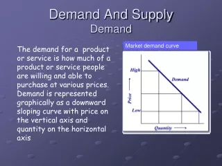
Demand • Demand Curve and Demand Schedule • The term demand refers to the entire relationship between the price of the good and quantity demanded of the good. • A demand curve shows the relationship between the quantity demanded of a good and its price when all other influences on consumers’ planned purchases remain the same.
Demand • Figure 3.1 shows a demand curve for energy bars. • A rise in the price, other things remaining the same, brings a decrease in the quantity demanded and a movement along the demand curve.
Demand • Willingness and Ability to Pay • A demand curve is also a willingness-and-ability-to-pay curve. • The smaller the quantity available, the higher is the price that someone is willing to pay for another unit. • Willingness to pay measures marginal benefit.
Demand • A Change in Demand • When some influence on buying plans other than the price of the good changes, there is a change in demand for that good. • The quantity of the good that people plan to buy changes at each and every price, so there is a new demand curve. • When demand increases, the demand curve shifts rightward. • When demand decreases, the demand curve shifts leftward.
Demand • Six main factors that change demand are • The prices of related goods • Expected future prices • Income • Expected future income • Population • Preferences
Demand • Prices of Related Goods • A substitute is a good that can be used in place of another good. • A complement is a good that is used in conjunction with another good. • When the price of substitute for an energy bar rises or when the price of a complement of an energy bar falls, the demand for energy bars increases.
Demand • Expected Future Prices • If the price of a good is expected to rise in the future, current demand fore the good increases and the demand curve shifts rightward. • Income • When income increases, consumers buy more of most goods and the demand curve shifts rightward. A normal good is one for which demand increases as income increases. An inferior good is a good for which demand decreases as income increases.
Demand • Expected Future Income • When income is expected to increase in the future, the demand might increase now. • Population • The larger the population, the greater is the demand for all goods. • Preferences • People with the same income have different demands if they have different preferences.
Demand • A Change in the Quantity Demanded Versus a Change in Demand • Figure 3.3 illustrates the distinction between a change in demand and a change in the quantity demanded.
Demand • A Movement along the Demand Curve • When the price of the good changes and everything else remains the same, the quantity demanded changes and there is a movement along the demand curve.
Demand • A Shift of the Demand Curve • If the price remains the same but one of the other influences on buyers’ plans changes, demand changes and the demand curve shifts.
Supply • If a firm supplies a good or service, then the firm • 1. Has the resources and the technology to produce it, • 2. Can profit from producing it, and • 3. Has made a definite plan to produce and sell it. • Resources and technology determine what it is possible to produce. Supply reflects a decision about which technologically feasible items to produce. • The quantity supplied of a good or service is the amount that producers plan to sell during a given time period at a particular price.
Supply • The Law of Supply • The law of supply states: • Other things remaining the same, the higher the price of a good, the greater is the quantity supplied; and • the lower the price of a good, the smaller is the quantity supplied. • The law of supply results from the general tendency for the marginal cost of producing a good or service to increase as the quantity produced increases (Chapter 2, page 37). • Producers are willing to supply a good only if they can at least cover their marginal cost of production.
Supply • Supply Curve and Supply Schedule • The term supply refers to the entire relationship between the quantity supplied and the price of a good. • The supply curve shows the relationship between the quantity supplied of a good and its price when all other influences on producers’ planned sales remain the same.
Supply • Figure 3.4 shows a supply curve of energy bars. • A rise in the price of an energy bar, other things remaining the same, brings an increase in the quantity supplied.
Supply • Minimum Supply Price • A supply curve is also a minimum-supply-price curve. • As the quantity produced increases, marginal cost increases. • The lowest price at which someone is willing to sell an additional unit rises. • This lowest price is marginal cost.
Supply • A Change in Supply • When some influence on selling plans other than the price of the good changes, there is a change in supply of that good. • The quantity of the good that producers plan to sell changes at each and every price, so there is a new supply curve. • When supply increases, the supply curve shifts rightward. • When supply decreases, the supply curve shifts leftward.
Supply • The five main factors that change supply of a good are • The prices of productive resources • The prices of related goods produced • Expected future prices • The number of suppliers • Technology
Supply • Prices of Productive Resources • If the price of resource used to produce a good rises, the minimum price that a supplier is willing to accept for producing each quantity of that good rises. • So a rise in the price of productive resources decreases supply and shifts the supply curve leftward.
Supply • Prices of Related Goods Produced • A substitute in production for a good is another good that can be produced using the same resources. • The supply of a good increases if the price of a substitute in production falls. • Goods are complements in production if they must be produced together. • The supply of a good increases if the price of a complement in production rises.
Supply • Expected Future Prices • If the price of a good is expected to rise in the future, supply of the good today decreases and the supply curve shifts leftward. • The Number of Suppliers • The larger the number of suppliers of a good, the greater is the supply of the good. An increase in the number of suppliers shifts the supply curve rightward.
Supply • Technology • Advances in technology create new products and lower the cost of producing existing products, so advances in technology increase supply and shift the supply curve rightward. • A natural disaster is a negative technology change, which decreases supply and shifts the supply curve leftward.
Supply • Figure 3.5 shows an increase in supply. • An advance in the technology for producing energy bars increases the supply of energy bars and shifts the supply curve rightward.
Supply • A Change in the Quantity Supplied Versus aChange in Supply • Figure 3.6 illustrates the distinction between a change in supply and a change in the quantity supplied.
Supply • A Movement Along the Supply Curve • When the price of the good changes and other influences on sellers’ plans remain the same, the quantity supplied changes and there is a movement along the supply curve.
Supply • A Shift of the Supply Curve • If the price remains the same but some other influence on sellers’ plans changes, supply changes and the supply curve shifts.
Market Equilibrium • Equilibrium is a situation in which opposing forces balance each other. Equilibrium in a market occurs when the price balances the plans of buyers and sellers. • The equilibrium price is the price at which the quantity demanded equals the quantity supplied. • The equilibrium quantity is the quantity bought and sold at the equilibrium price. • Price regulates buying and selling plans. • Price adjusts when plans don’t match.
Market Equilibrium • Price as a Regulator • Figure 3.7 illustrates the equilibrium price and equilibrium quantity. • If the price is $2.00 a bar, the quantity supplied exceeds the quantity demanded. • There is a surplus of 6 million energy bars.
Market Equilibrium • If the price is $1.00 a bar, the quantity demanded exceeds the quantity supplied. • There is a shortage of 9 million energy bars. • If the price is $1.50 a bar, the quantity demanded equals the quantity supplied. • There is neither a shortage nor a surplus of energy bars.
Market Equilibrium • Price Adjustments • At prices above the equilibrium price, a surplus forces the price down. • At prices below the equilibrium price, a shortage forces the price up. • At the equilibrium price, buyers’ plans and sellers’ plans agree and the price doesn’t change until some event changes either demand or supply.
Predicting Changes in Price and Quantity • An Increase in Demand • Figure 3.8 shows that when demand increases the demand curve shifts rightward. • At the original price, there is now a shortage. • The price rises, and the quantity supplied increases along the supply curve.
Predicting Changes in Price and Quantity • An Increase in Supply • Figure 3.9 shows that when supply increases the supply curve shifts rightward. • At the original price, there is now a surplus. • The price falls, and the quantity demanded increases along the demand curve.
Predicting Changes in Price and Quantity • Change in Demand with No Change in Supply • When demand increases, equilibrium price rises and theequilibrium quantity increases.
Predicting Changes in Price and Quantity • Change in Demand with No Change in Supply • When demand decreases, the equilibrium price falls and the equilibrium quantity decreases.
Predicting Changes in Price and Quantity • Change in Supply with No Change in Demand • When supply increases, the equilibrium price falls and theequilibrium quantity increases.
Predicting Changes in Price and Quantity • Change in Supply with No Change in Demand • When supply decreases, the equilibrium price rises and theequilibrium quantity decreases.
Predicting Changes in Price and Quantity • Increase in Both Demand and Supply • An increase in demand and an increase in supply increase the equilibrium quantity. • The change in equilibrium price is uncertain because the increase in demand raises the equilibrium price and the increase in supply lowers it.
Predicting Changes in Price and Quantity • Decrease in Both Demand and Supply • A decrease in both demand and supply decreases the equilibrium quantity. • The change in equilibrium price is uncertain because the decrease in demand lowers the equilibrium price and the decrease in supply raises it.
Predicting Changes in Price and Quantity • Decrease in Demand and Increase in Supply • A decrease in demand and an increase in supply lowers the equilibrium price. • The change in equilibrium quantity is uncertain because the decrease in demand decreases the equilibrium quantity and the increase in supply increases it.
Predicting Changes in Price and Quantity • Increase in Demand and Decrease in Supply • An increase in demand and a decrease in supply raises the equilibrium price. • The change in equilibrium quantity is uncertain because the increase in demand increases the equilibrium quantity and the decrease in supply decreases it.
捷運路線房地產價格變化 • 台北捷運通車以來,包括木柵線、淡水線、新店線、中永和線及板南線等,正式通車後,對附近房地產市場都出現顯著的發酵,改變都會區運輸結構,民眾可享更便捷交通環境;而在捷運周邊的住宅房價,仍以北市精華地段獲益較明顯,而部分屬高架主體的捷運站,如文山區、淡水線等漲幅較小。房地產業者表示,最早完工通車的木柵線,因屬高架設計,所經路段如大安、中山地區,也是北市的精華區之一,而通車後,也讓包括市區的忠孝復興至大安站一帶的房價居高不下。而木柵線停靠站多的文山區,對房價的提昇,相對與一般行情,成長幅度明顯較小,原因在於全線採高架建構,對購屋者而言,認為不算利多,但在前幾年房市低迷時,該地區捷運站周邊的房價,下降幅度亦不大,抗跌力不弱。
捷運路線房地產價格變化 • 至於在86年完工的淡水新店線,與88年通車的小南門、新北投支線,該路線目前行經路段最長,而且是高架、平面、地下三者兼具;而該路線對台北市中正區各站的房價激勵最明顯,租售報導指出,在通車半年後,中正紀念堂周邊的預售屋,漲幅超過6%,而新成屋更達約10%;古亭站也有約5%漲幅;目前房價仍屬高檔。 文山地區各站房價,在區域行情下跌時,仍能維持不墜;而該捷運的通車,對偏遠的新店地區,是為大利多;目前新店線各捷運站週邊的房價,都比區域內行情,高出5%至10%。 在往淡水路線部分,在市區內的雙連、中山與民權西路各站,周邊房價也有不小的漲幅,平均都有一成上下,但愈往淡水方向,漲幅愈低。
捷運路線房地產價格變化 • 板橋南港線通車後,同樣造成各站週邊房價的炒作,在北市區的大安、及信義區各站,由於位居市區精華地段行情備受哄抬,業者說,從忠孝新生站至永春站一帶,比區域內行情高出一至一成五。這是可供消費者參考的實例。 板南線目前在板橋地區,僅有江子翠站與新埔站,而板橋地區過去幾年的行情,每坪大致都在20萬元以下,甚至有下跌的窘境,但在捷運通車之後,車站週邊行情每坪超過25萬元已不稀奇。而板南線將經過土城,延伸至三峽、鶯歌地區,對沿線房房價有助漲效果。