Download
1 / 41
410 likes | 514 Views
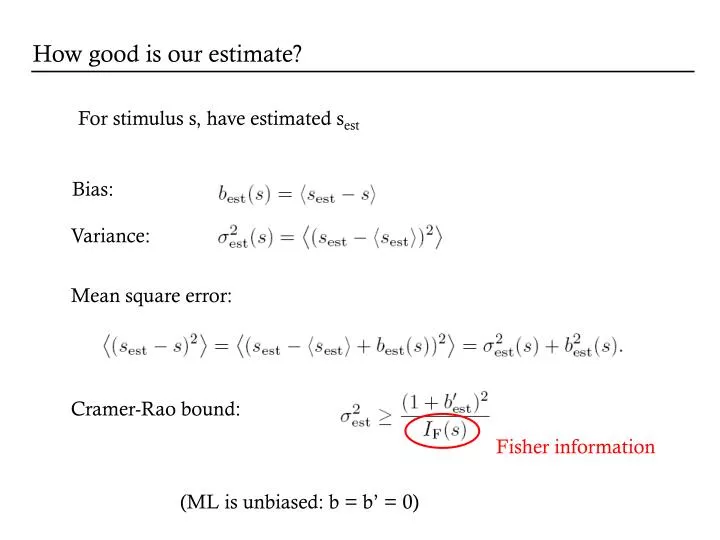
How good is our estimate? . For stimulus s , have estimated s est. Bias: . Variance:. Mean square error:. Cramer- Rao bound:. Fisher information. (ML is unbiased: b = b ’ = 0). Fisher information. Alternatively:. Quantifies local stimulus discriminability.

E N D
How good is our estimate? For stimulus s, have estimated sest Bias: Variance: Mean square error: Cramer-Rao bound: Fisher information (ML is unbiased: b = b’ = 0)
Fisher information Alternatively: Quantifies local stimulus discriminability
Fisher information for Gaussian tuning curves For the Gaussian tuning curves w/Poisson statistics:
Fisher information and discrimination Recall d' = mean difference/standard deviation Can also decode and discriminate using decoded values. Trying to discriminate s and s+Ds: Difference in ML estimate is Ds (unbiased) variance in estimate is 1/IF(s).
Limitations of these approaches • Tuning curve/mean firing rate • Correlations in the population
Entropy and information For a random variable X with distribution p(x), entropy is given by H[X] = - Sxp(x) log2p(x) Information is defined as I[X] = - log2p(x)
Maximising information Binary distribution: Entropy Information
Entropy and information Typically, “information” = mutual information: how much knowing the value of one random variable r (the response) reduces uncertainty about another random variable s (the stimulus). Variability in response is due both to different stimuli and to noise. How much response variability is “useful”, i.e. can represent different messages, depends on the noise. Noise can be specific to a given stimulus.
Entropy and information Information quantifies how independent r and s are: I(s;r) = DKL [P(r,s), P(r)P(s)] Alternatively: I(s;r) = H[P(r)] – Ss P(s) H[P(r|s)] .
Entropy and information Information is the difference between the total response entropy and the mean noise entropy: I(s;r) = H[P(r)] – Ss P(s) H[P(r|s)] . Need to know the conditional distribution P(s|r) or P(r|s). Take a particular stimulus s=s0 and repeat many times to obtain P(r|s0). Compute variability due to noise: noise entropy
Entropy and information Information is symmetric in r and s Examples: response is unrelated to stimulus: p[r|s] = p[r] response is perfectly predicted by stimulus: p[r|s] = d(r-rs)
Information in single cells: the direct method How can one compute the entropy and information of spike trains? Discretize the spike train into binary words w with letter size Dt, length T. This takes into account correlations between spikes on timescales TDt. Compute pi = p(wi), then the naïve entropy is Strong et al., 1997; Panzeri et al.
Information in single cells: the direct method Many information calculations are limited by sampling: hard to determine P(w) and P(w|s) Systematic bias from undersampling. Correction for finite size effects: Strong et al., 1997
Information in single cells: the direct method Information is the difference between the variability driven by stimuli and that due to noise. Take a stimulus sequence sand repeat many times. For each time in the repeated stimulus, get a set of words P(w|s(t)). Should average over all s with weight P(s); instead, average over time: Hnoise = < H[P(w|si)] >i. Choose length of repeated sequence long enough to sample the noise entropy adequately. Finally, do as a function of word length T and extrapolate to infinite T. Reinagel and Reid, ‘00
Information in single cells Fly H1: obtain information rate of ~80 bits/sec or 1-2 bits/spike.
Information in single cells Another example: temporal coding in the LGN (Reinagel and Reid ‘00)
Information in single cells Apply the same procedure: collect word distributions for a random, then repeated stimulus.
Information in single cells Use this to quantify how precise the code is, and over what timescales correlations are important.
Information in single spikes How much information does a single spike convey about the stimulus? Key idea: the information that a spike gives about the stimulus is the reduction in entropy between the distribution of spike times not knowing the stimulus, and the distribution of times knowing the stimulus. The response to an (arbitrary) stimulus sequence s is r(t). Without knowing that the stimulus was s, the probability of observing a spike in a given bin is proportional to , the mean rate, and the size of the bin. Consider a bin Dt small enough that it can only contain a single spike. Then in the bin at time t,
Now compute the entropy difference: prior conditional and using Assuming , In terms of information per spike (divide by ): Information in single spikes , Note substitution of a time average for an average over the r ensemble.
Information in single spikes Given • note that: • It doesn’t depend explicitly on the stimulus • The rate r does not have to mean rate of spikes; rate of any event. • Information is limited by spike precision, which blurs r(t), • and the mean spike rate. Compute as a function of Dt: Undersampled for small bins
Synergy and redundancy The information in any given event can be computed as: Define the synergy, the information gained from the joint symbol: or equivalently, Negative synergy is called redundancy.
Exmple: multispikepatterns In the identified neuron H1, compute information in a spike pair, separated by an interval dt: Brenner et al., ’00.
Using information to evaluate neural models We can use the information about the stimulus to evaluate our reduced dimensionality models.
Evaluating models using information Mutual information is a measure of the reduction of uncertainty about one quantity that is achieved by observing another. Uncertainty is quantified by the entropy of a probability distribution, ∑ p(x) log2p(x). We can compute the information in the spike train directly, without direct reference to the stimulus (Brenner et al., Neural Comp., 2000) This sets an upper bound on the performance of the model. Repeat a stimulus of length T many times and compute the time-varying rate r(t), which is the probability of spiking given the stimulus.
Evaluating models using information Information in timing of 1 spike: By definition
Evaluating models using information Given: By definition Bayes’ rule
Evaluating models using information Given: By definition Bayes’ rule Dimensionality reduction
Evaluating models using information Given: By definition Bayes’ rule Dimensionality reduction So the information in the K-dimensional model is evaluated using the distribution of projections:
Compute modes and projections … A1 B A2 B A3 B Compute mean rate Experimental design Alternate random and repeat stimulus segments:
Using information to evaluate neural models Here we used information to evaluate reduced models of the Hodgkin-Huxley neuron. Twist model 2D: two covariance modes 1D: STA only
Information in 1D The STA is the single most informative dimension.
Information in 1D • The information is related to the eigenvalue of the corresponding eigenmode • Negative eigenmodes are much more informative • Information in STA and leading negative eigenmodes up to 90% of the total
Information in 2D • We recover significantly more information from a 2-dimensional description
Information in 2D Information captured by 2D model Information captured by STA
Synergy in 2 dimensions Get synergy when the 2D distribution is not simply a product of 1D distributions The second dimension contributes synergistically to the 2D description: the information gain >> the information in the 2nd mode alone
Other fascinating subjects Adaptive coding: matching to the stimulus distribution for efficient coding Maximisinginformation transmission through optimal filtering predicting receptive fields Populations: synergy and redundancy in codes involving many neurons multi-information Sparseness: the new efficient coding