Download
1 / 32
320 likes | 469 Views
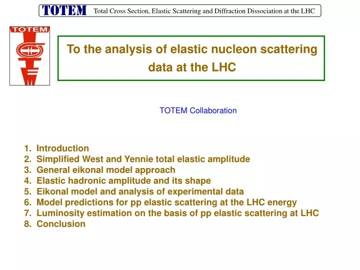
To the analysis of elastic nucleon scattering data at the LHC. TOTEM Collaboration. 1. Introduction 2. Simplified West and Yennie total elastic amplitude 3. General eikonal model approach 4. Elastic hadronic amplitude and its shape 5. Eikonal model and analysis of experimental data

E N D
To the analysis of elastic nucleon scattering data at the LHC TOTEM Collaboration 1. Introduction 2. Simplified West and Yennie total elastic amplitude 3. General eikonal model approach 4. Elastic hadronic amplitude and its shape 5. Eikonal model and analysis of experimental data 6. Model predictions for pp elastic scattering at the LHC energy 7. Luminosity estimation on the basis of pp elastic scattering at LHC 8. Conclusion
1. Introduction Elastic nucleon collisions at high energies: • hadronic interactions at all t&Coulomb scattering mainly at small |t| • influence of both interactions (spins neglected)(Bethe (1958)) pp at plab = 24 ÷ 2900 GeV/c FC+N(s,t) = FC(s,t) e i αΦ(s,t) + FN(s,t) • FC(s,t) … Coulomb (QED), • FN(s,t) …hadronic (unknown) αΦ(s,t) … relative phase; α=1/137.036 … fine structure constant • no theory of hadronic interactions at small |t|→ looking for phenomenological shape from data 2
two unknown functions:FN(s,t) , Φ(s,t) • West and Yennie (1968) • common belief: WY quite general … valid for any shape of t • however:V.K. & M. Lokajíček, Phys. Lett. B 611 (2005) 102, V.K., M. Lokajíček & I. Vrkoč, Phys. Lett. B656 (2007) 182 WY may be regularly applied only toFN(s,t) having ρ(s,t) = Re FN(s,t) Im FN(s,t) = ρ(s) = const at all kinematically allowedt values (otherwiseΦ(s,t) complex) 3
2. Simplified West -Yennie total elastic amplitude • derived for: • ρ = const …..for all kinematically allowed t • |F N(s,t)|= eBt/2… B = const …for all kinematically allowed t • applied high-energy approximations • (V.K. & M. Lokajíček, Phys. Lett. B 611 (2005) 102) used:|t| ≤ .01 GeV 2 ; higher |t| … Coulomb scatt. neglected → inconsistent use (V.K. & M. Lokajíček, Phys. Lett. B 232 (1989) 263) both assumptions not fulfilled (theoretically & experimentally) 4
3. General eikonal model approach • previous eikonal models based on approximate form of Fourier-Bessel transformation valid at asymptotic s and small |t| • mathematically rigorous formulation (valid at anysandt)(Adachi et al., Islam (1965 – 1976)) additivity of pottentials additivity of eikonals (Franco (1973), Cahn (1982)) δC(s,b) … Coulomb eikonal δN(s,b) … hadronic eikonal δC+N(s,b) … total eikonal • total elastic amplitude 5
convolution integral • equation describes simultaneous actions of both Coulomb and hadronic interactions; to the sum of both amplitudes new complex function (convolution integral) is added─ at difference to WY amplitude (Coulomb amplitude multiplied by phase factor only) • valid at any s and t 6
total scattering amplitude valid up to terms linear inα • and for small |t| ... for any shape of t (Cahn 1982) • used in: V.K., M. Lokajíček & D. Krupa: Phys. Rev. D35 (1987) 1719; • D41(1990) 1687; D46 (1992) 4087 • limitation for small |t| removed: • V. K. & M. Lokajíček, Z. Phys. C63 (1994) 619 7
total scattering amplitude valid up to terms linear inαfor any t B(s,t) & ρ(s,t) …exact 8
advantage: analytical calculation of I(t,t’) • form factors (Borkowski et al (1975)) → → • only one integration over t’ remains • either for analysis of data or for model predictions 9
Elastic hadronic amplitude and its shape (i) Dominance of imaginary part • common approach: dominant Im FN(s,t)in broad interval of |t|→phase increases with increasing |t| and Im FN(s,tdiff)=0;Re FN(s,t)increases with increasing |t| to obtain non-zero dσ/dt at tdiff ; Re FN(s,tdiff)≠0. • diffractive minimum → minimum of the squares of both real and imaginary parts → theoretically no need for Im FN(s,tdiff)=0 • van Hove (1963): dominance of imaginary part only at asymptotic energies and very small |t|;V.K., M. Lokajíček: Mod. Phys. Lett.11 (1996) 2241 → dominance hardly justified in broad region of t • Auberson, Kinoshita & Martin (1971), Martin (1973): • asymptotic s and infinitesimally small t(geometrical scaling) . Φ(τ) … real entire function of V.K., M. Lokajíček: Phys. Rev. D31 (1985) 1045; D55 (1997) 3221 Φ(τ) … becomes complex for |t| ≥ 0.15 GeV2 pp ISR 10
→dominance of Im FN(s,t) … justified only at very small |t| (ii) t dependence at small |t| • elastic hadronic amplitudeFN(s,t) (strong interactios) → conservation of isospin(Heisenberg (1932), M. Lokajíček &V. Votruba (1953)) • NN scattering… isospin states (Clebsch-Gordan coeff.) • |NN>≡|j1 j2;m1m2>=| j1j2;JM><j1j2;JM|j1j2;m1m2> • |pp>=|½½;11>, |np>= ½ |½½;10> + ½ |½½;00>, • |nn>=|½½;1-1> • isospin conservation: • <I I3|FN(s,t)|I’ I3’> = F2I(s,t)δII’δI3 I3’ • <pp|FN(s,t)|pp> = F2 (s,t), <np|FN(s,t)|np> = ½ F2(s,t) + ½F0(s,t) • <np|Fch.e.(s,t)|pn> = ½ [F2(s,t) – F0(s,t)] → 11
consequence of isospin conservation (valid at anysandt ) Fch.e.(s,t) = FNpp(s,t) – FNnp(s,t) • data ( plab ~ 300 GeV/c) pp [Burq et al: Nucl. Phys. B217 (1983) 285], np [Arefiev et al: Nucl. Phys. B232 (1984) 365) np → pn [Barton et al: Phys. Rev. Lett. 37(1976) 1656, 1659 Landolt-BornsteinVol. 9, Springer 1980] • (pp)el (total)(np)el np → pn • -t [GeV2]dσ/dt [mb/GeV2]dσ/dt [mb/GeV2]dσ/dt [μb/GeV2] • .003 103.34 ± 4.1 77.09 ± .80 6.14 ± .006 • .023 58.27 ± 1.1 61.80 ± .71 4.24 ± .004 • → dσ/dt [np → pn] ~ 10 -4 dσ/dt[np] • → FNpp(s,t) ≡ FNnp(s,t) [~1%] • np measured up to|t |~ 10 -5 GeV2→ |FN(s,t)| ~ e-Bt/2 12
(iii) mean-squares of impact parameter in nucleon collisions • eikonal model: enables to analyze impact parameter distributions corresponding to different kinds of hadronic collisions (mean squares) • elastic mean square(V.K., M. Lokajíček Jn., M. Lokajíček Sn., Czech. J. Phys. B 31 (1981) 1334; V.K., M. Lokajíček, D. Krupa, Phys. Lett. B 544 (2002) 132) Heney & Pumplin (1976) • first term: contribution of modulus • second term: contribution of derivative ζN ’(s,t)… neglected if WY integral formula for relative phase (caused by ζN(s,t)=const) is used → fundamental limitation !!! 13
two cases: • if ζN’ (s,t) >> 0at small |t|→ peripheral distribution • if ζN’ (s,t) ~ constat small |t| → central distribution • similar strong t dependence of ζN(s,t):(Franco &Yin (1985,1986)) • central distribution: artificial discrepancy between elastic and single diffractive collisions (always considered as peripheral; e.g., Kane (1972), Sakai & White (1973), Humble (1973), Cohen-Tannudji, Maor (1975), Chou-Yang (1985), … • discrepancy removed if elastic collisions are peripheral (smaller χ2 ) 14
total mean square • inelastic mean square (iv) impact parameter profiles Adachi & Kotani (1965-1976) 16 papers, Islam (1968,1976) • added in the unphysical region; required by mathematics of FB transformation • similarly also FB transformation of inelastic overlap function ginel(s,b) 15
unitarity condition • oscillations at higher b ; can be removed by adding c(s,b) fulfilling some • conditions (V.K., M. Lokajíček, D. Krupa, Proceedings of IX. Blois Workshop • 2001; Phys. Lett. B 544 (2002) 132; Czech. J. Phys. 53 (2003) 645) • modified unitarity condition (“diagonal”) ↑ ↑ ↑ central peripheral central (v) central and peripheral behaviors of elast.hadronic scatt. • central: large transparency of proton in ‘head-on collisions’ (Miettinen (1974) … ‘puzzle’ (Giacomelli & Jacob (1979)); artefact based on a priori assumption … can be removed if elast. hadronic scatt. is peripheral (V.K. & Lokajíček (1981,…) • peripheral: steep increase of ξN‘(s,t) at small |t| (necessary but not sufficient condition) 16
Fig. 3: original oscillating profiles (statistical errors) • Fig. 9: final shape of profiles; full lines: red … peripheral elastic profile • green … central total profile • yellow … central inelastic profile • “original” values of total, elastic and inelastic rms and of cross sections conserved 17
5. Eikonal model and analysis of experimental data • modulus and phase of phase ξN(s,t) parameterized (at all t ) … peripheral … central 18
Results (pp at 53 GeV, ppbar at 541 GeV)(V. K. & M. Lokajíček, Z. Phys. C63 (1994) 619) • dσ/dt well decsribed for peripheral as well as central cases; peripheral preferred • values of σtot , B(t) , ρ(t) slightly different from standard WY analysis at t=0 • B(t), ρ(t) at all t determined for the first time • ratio of interference to hadronic terms increases at some higher |t| → influence • of Coulomb scattering cannot be neglected at higher |t| • values of root-mean-squares and shapes of all profiles obtained for the first time • central case: elast. rms lesser than inelastic rms pp scatt. at 53 GeV (J. Procházka, batcheler thesis, Charles Univ. Prague, 2007) 19
6. Model predictions for pp elastic scattering at the LHC energy COMPETE Collab.: fits to all available data; predictions based on DR technique PRL 89 201801 (2002) TOTEM aim: ~ 1% error of σtot model predictions: 90 ÷ 130 mb σtot = 125 ± 25 mb based on QCD (Landshoff, arXiv:0709.0395 [hep-ph] analyzed models: • M.M. Islam, R.J. Luddy and A.V. Prokudin: Phys. Lett. B605 (2005) 115 • V.A. Petrov, E. Predazzi and A.V. Prokudin: Eur. Phys. J. C28 (2003) 525 • C. Bourrely, J. Soffer and T.T. Wu: Eur. Phys. J. C28 (2003) 97 • M.M. Block, E.M. Gregores, F. Halzen and G. Pancheri: Phys. Rev. D60 (1999) 0504024 20
results of model analysis (eikonal total amplitude) modelσtot [mb] σel[mb] B(0) [GeV-2]ρ <btot2>1/2 [fm] < bel2>1/2[fm] <binel2>1/2 [fm] Islam 109.17 21.99 31.43 0.123 1.552 1.048 1.659 Petrov et al. 2P 94.97 23.94 19.34 0.0968 1.227 0.875 1.324 Petrov et al. 3P 108.22 29.70 20.53 0.111 1.263 0.901 1.375 BSW 103.64 28.51 20.19 0.121 1.249 0.876 1.399 Block Halzen 106.74 30.66 19.35 0.114 1.223 0.883 1.336 • all root-mean-squares can be estimated if elastic hadronic amplitude FN(s,t), i.e., the modulus|FN(s,t)| and the phaseζN(s,t), are known • elastic rms are lesser than inelastic ones → hadron elastic nucleon collisions are more • central than the inelastic nucleon collisions → ‘puzzle’ 21
model hadronic amplitudes in forward direction – predictions of total cross section values • TOTEM σtot = ? … model selection • integral dispersion relations → prediction at higher energies 22
differential cross section at higher|t|values ppISR53 GeV (plotted with the same values of fitted parameters) pp 14 TeV LHC • diffractive structure? only one diffractive minimum? • values of at higher|t|values? • TOTEM … selection of models 23
tdependence of diffractive slopeB(t) at LHC • V.K., M. Lokajíček, D. Krupa, Phys. Rev. D16 (1990) 1687; ibid D41 (1992) 1687 • V.K., M. Lokajíček, Z. Phys. C63 (1994) 619 • different model predictions • typical tdependence (similar as in pp scattering at the ISR) observed • TOTEM: selection of models 24
ρ(t) modeldependence • ρ(t) is not constant • justification for the use of total eikonal model amplitude • (neded for consistent description of influence of Coulomb interaction) 25
interference term • can be hardly neglected at higher|t| (as in WY approach) • justification for eikonal total amplitude 26
7. Luminosity estimation on the basis of pp elast. scatt. at LHC • different total (eikonal and WY) amplitudes different luminosity determinations • pp 14 TeV • luminosity determined with large systematic error if WY approach used !!! • correct estimation of luminosity if eikonal approach used at any t eikonal WY 27
difference between eikonal and WY total amplitudes (for given models) • at the LHC • if luminosity is specified with the help of elastic scatt. in the center of interference region on the basis of WY total amplitude → it will be determined with 5 % systematic error • correct description of Coulomb – hadronic interference needed 28
(vi) scattering in very forward direction • center of interference region (WY ampl.): • |Fc(s,t)| = |FN(s,t)| → |t| ~ 8 πα / σtot = 0.071 / σtot(mb) • 53 GeV: .0016 GeV2 • 14 TeV: .00051 GeV2 • interference “window” becomes narrower when energy increases → measurement at very small|t| …technically very hard to perform • tradition (WY ampl.):σtot , B(0), ρ(0) • new analysis (eikonal):σtot ,B(t), ρ(t) • data admit roughly exponential t dependence → flexible parameterizations of the modulus and of phase are needed 29
8. Conclusion • WY integral formula:onlyhadronic amplitudes with constant ρ • eikonal model suitable tool for analyzing elastic hadron amplitudet dependence of modulus and phase needed at all measured t • dynamical characteristics of elastic hadronic amplitude determinedby itst dependence σtot , ρ(t), B(t) … model dependent quantities • luminosity: correct estimation if eikonal approach used TOTEM experiment: • (i) to determine in the most precise way (ii) construction of elastic hadronic amplitude FN(s,t) (iii) estimation of σtot , B(t), ρ(t), luminosity (iv) selection of model predictions … very useful tool 30
root-mean-squares: elastic: total: inelastic:
items (in theory) to be solved • integral dispersion relations • actual shapes of profiles (statistical errors) • model of peripheral elastic hadronic scattering • numerical programs (in C++) • Pumplin’s bound and modifications of Thomas – Miettinen parton model of diffractive dissociation