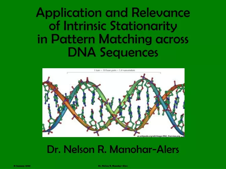
Application and Relevance of Intrinsic Stationarity in Pattern Matching across DNA Sequences

1. Application and Relevance of Intrinsic Stationarity in Pattern Matching across DNA Sequences Dr. Nelson R. Manohar-Alers en.wikipedia.org/wiki/Image:DNA_Overview.png Dr. Nelson R. Manohar-Alers

2. Background • Advanced Intelligent Networks (ATT, 87-90) • Statistical Process Control (IOE, 91-92) • Software Systems Research (CSE, 92-97) • Asynchronous Groupware • Multimedia Scheduling and Synchronization • Adaptive Resource Management (IBM, 97-01) • Adaptive Rate Control • Estimation of Performance Envelopes • Adaptive Internet Resource and Capacity Shaping • Bioinformatics (HPS, present) • HPS Measurements and Approximation • HPS Feature Extraction • HPS Pattern Matching • DNA Homology and Sequence Alignment Dr. Nelson R. Manohar-Alers

3. Some Basic DNA Concepts • Genome, chromosomes, genes, nucleotides (4 DNA-bases) • genes are protein encoding instructions • ~30K genes in human genome • encoded as sequences of nucleotides • AT/CG pairs, double helix structure (Watson-Crick) • Comparative Genomics • discovery of structure on nucleotide sequences • discovery of interactions and regulatory networks/functions • Bioinformatics • algorithms for genomic analysis • homology, sequence alignment, phylogenomics, etc. • mining of APPROXIMATE SIMILARITY across DNA sequences • nucleotides: adenine (A), cytosine (C), guanine (G), thymine(T) • 3x109 base pairs (bp) • 1-p (95-97%) non-coding (buffer, junk) DNA, p (3-5%) coding sequences (genes) • large % of junk DNA may be functional/structurally important (conserved DNA) • amino acids: triplets of mRNA (A, C, G, T/U) transcribed into 20 amino acids • alanine (A), aspartic acid (D), glutamic acid (E), glutamine (Q), lysine (K), etc… Dr. Nelson R. Manohar-Alers

4. Importance of DNA Similarity Mining • Sequence alignment and similarity mining • represent fundamental algorithmic BUILDING BLOCKS in bioinformatics • Why? • inferred homologues in comparative genomics • sequences that are similar may be related in FUNCTION, EVOLUTION, … • inferred evolutionary distance in molecular phylogenomics • evolutionary relevance of inserts/deletes (indels) (mutated/noisy DNA) • Increased query sophistication and query size • identification of features in DNA (23ANDME) • screening of DNA sequence against DNA databases • comparative genomics for very large sequences (e.g., genomes) • large-scale similarity interrupted by structural rearrangement of regions of local similarity • (Delcher, Kasif, Fleischmann, Peterson, White, Salzberg, 1999) • AND DB SIZE! – DNA databank growth is exponential • new genomes/sequences added constantly • 65x109 bp, 61x106 sequences 80x109 bp, 18x106 sequences (Jan 08, NCBI) • relationships of new sequences/genomes to existing ones? en.wikipedia.org/ wiki/GenBank Dr. Nelson R. Manohar-Alers

5. Approximate Similarity: Basic Ideas signature S A T G T A C A C A C A C C G C G A C C G A T A T C T G A G T A T G T A A T A T T A T G T C T A C T • Similarity Mining of Approximate Homologue Instance H(k) of S in T • Inputs: • signature S and a target sequence T • T/S size ratio can be orders of magnitude (e.g., sequence, genome, etc) • Goal: • find SUFFICIENTLY SIMILAR sequence(s) (H(k)) of a signature S in a target sequence T • Constrained by: (some f().edit_distance): • mismatches (single-point errors without affecting sequence alignment) • indels – burst of extraneous/missing DNA bases which affect alignment • possibly, structural re-arrangements or transpositions of subsequences within • Key Concepts: • discovery of some structure/pattern that CLUES local/global alignment and similarity • Output: • SIMILARITY alignment of each approximate homologue H(k) to S • DIFFERENTIATION relationships between homologues and signature • Biological Sequences and (Approximate) Substring Search • 1970s well-established field (Knuth-Morris-Pratt, Boyer-Moore, Aho, …) • relevance of edit distance constraints (mismatches, substitutions, and indels) • relevance of conserved and non-conserved regions • local, global, and glocal similarity algorithms A T G T A C A C G C A C A G C G A C C G C T A A T A T C T G A A T G T A A T A T T A T G T C T A C homologue H(k) of S in T f().insert/delete (indel) f().segment f().mismatches Dr. Nelson R. Manohar-Alers

6. Optimal Local Sequence Alignment • Smith-Waterman (id, J Mol Biol 1981, 147(1):195-197) • dynamic programming algorithm • MODERATE sequence sizes, handling of inserts and mismatches • optimal local alignment between two sequences in O(N·M) time • setups a tableaux • N columns of the target sequence • M rows of the signature sequence • populates tableaux using adjacency recurrences • computes for all positions in tableaux, score based on recurrences • row-adjacent (indel/gap penalty) • column-adjacent (indel/gap penalty) • diagonal cells traversals (match bonus) • adds/subtracts from accumulative traversal score with • bonus (larger weight) • match bonus (e.g., 1) • penalties (different weight) • mismatch penalty (e.g., 0.3) • gap penalty (e.g., 1.3) • identifies optimal local alignments • as backward traversal from global maximal score • through local adjacency maximal scores SMITH-WATERMAN CAGCCUCGCUUAG  ...CAGCC–UCG... AAUGCCAUUGACGG  AAUGCCAUUG… Dr. Nelson R. Manohar-Alers

7. Faster, Heuristic-Based Local Alignment • BLAST (Myers, Altschul, Gish, Lipman, Miller, J. Mol. Biol. 1990, 215:403-410) • A global similarity should exhibit statistically-significant (i.e., distinguishable from noise) patterns of local similarity, then • compile list of seed/words from S • 1-st stage: find aligned pairs of such words between S and T • 2nd stage: extend • such micro-alignments (i.e., aligned word pairs) • into high-scoring local similarity regions (HSP/MSP) (i.e., with mismatches) • 3-rd stage: apply smith-waterman across said gapped regions (i.e., fast gapped alignment) • Key concepts: • BLAST (“fast gapped alignments”) is a very good idea • class of heuristic-based algorithms over conserved regions Dr. Nelson R. Manohar-Alers

8. Sensitivity, Speed, and Structure • Considerations w.r.t. a sampling word-based alignment • selection of word size (e.g., presence of mismatches within) • selection of words • resultant location distribution of said words (e.g., localization bias) • Create extrinsic glue or scaffolding structure (2nd Stage) • indexing aid such suffix tree or structural aid such as HMM • tradeoff speed/sensitivity if scaffolding structure and/or indexing used to examine the sequences • tradeoff speed/sensitivity if pattern(s) on words taken into account? • Sparse or alter the distribution of seeds (1st Stage) • more sensitivity at same speed; more speed at same sensitivity such as Pattern Hunter Dr. Nelson R. Manohar-Alers

9. PROPOSAL: Leverage Structural Intrinsic Property • Find some INTRINSIC PROPERTY (to be seed generator) that is • SUFFICIENTLY DENSE (but not too much, or with controllable density) • WELL-DISTRIBUTED throughout any sequence • efficient to REPRESENT (i.e., space) and efficient to COMPUTE (i.e., time) • Pattern-match over intrinsic structure instead of words/seeds • Stationary  “approximate lack of change” of certain statistical properties within a sequence • Could APPROXIMATE LACK OF CHANGE identify homologues? • SMOOTHS SMALL DIFFERENCES between sequences • for handling of mismatches or nucleotide polymorphisms (SNPs)? • UNEARTHS INTRINSIC STRUCTURAL FEATURES within a sequence • for the handling of indels differences? • ENABLES EFFICIENT COMPARISONS between sequences • for the handling of transpositions and re-arrangements? a time plot of “bursts of localized quasi-stationary conditions” Dr. Nelson R. Manohar-Alers

10. IAB IA {A} HPS signal (<n>micro-states) {B} IB input signal (Nsamples) {I*AB} {A} IA {B} {I*AB} Stationary-Based Approximations:The HPS Transform • Harmonic Process State (HPS) Transform • generates time series of <n> COARSE-GRAIN TRACKING micro-states • coupled with <n+1> FINE-TRACKING TRANSITIONS between these • research initially related to adaptive rate control [NRM98] decision-making between processes A and B based on HPS conditioned data I* decision-making between processes A and B based on non-conditioned data I • Robust simplification of DECISION-MAKING PROCESSES • homology analysis and sequence alignment are decision-making processes • approximate pattern match in (coarse-grain) HPS domain • transform back results into original fine-grain input domain Dr. Nelson R. Manohar-Alers

11. Local DNA DB Data Access Stub DNA DB Reader (S, T) Remote DNA DB HPS Transform (S, T) CoarseGrain Aligner(S, T) FineGrain Aligner(S, H(k)) Web Report Data Access Stub Report Generator (S, H(k)) Homology Pattern Mining in HPS Domain • Inputs • S: signature of size M • T: test sequence of size N • Goal • find all approximate homologues of S in T • accounting for mismatches, indels, bursts, & rearrangements* • Step 1: HPS Transform of S and T • representations of size m and n, respectively • where n«N and m«M • O(N+M) time • Step 2: Coarse Grain Aligner • combinatorial pattern matching • over shape of compressed representations • identifies all potential homologues H(i) of S in T • O(m2·n) time • Step 3: Fine Grain Aligner • given k potential homologues H(i) of S in T • verifies and aligns each H(i) to S • o(k·m2) worst case time • Output • up to k approximate homologues of S • all verified by reconstruction • precise location and alignment within T Alignment DNA DB High Level Software Architecture of HPS DNA Miner: Homology Features Dr. Nelson R. Manohar-Alers

12. Stationary Basic Idea “The Present” “similar” to “The Past”? Strictly Stationary P(zi<ai, … zk<ak) = P(zi+h<ai, … zk+h<ak), identical process everywhere, all moments are equal Wide Sense Stationary constant and finite variance, constant mean, covariance is function of the distance only Ergodic Process tau-invariance m(t)=m(t-t) of property m() measure stability of rate differential between long-term outlooks of signals law of large numbers, central limit Th. “Approximate” Wide Sense Stationary “LOCALIZED STATIONARY CONDITIONS” (finite bursts, stable mean and variance) quality of decision-making (signal de-noising, outliers ident. and handling) What’s Stationarity? What Flavor of It? y(t) µs(i) The Present? The Past? µf(i) t=i t Dr. Nelson R. Manohar-Alers

13. HPS Decision-Making Setup decision making setup at t=i • Is Present Similar Enough to Recent-Past? • recent past outlook (size m), present outlook (size m’) • same signal, outlooks from different times • loosely related to super-heterodyning (Armstrong, 1917) • Stationary ONLINE decision rule • if previous stationary bit is same as current stationary bit, • then (rule 1)  COARSE-TRACKING of signal • otherwise (rules 2, 3, 4)  FINE-TRACKING of the signal • generates stationary decision bit for present index • deceitfully clever test performed in O(1) time (i.e., using partial sums)! The Present The Recent Past HPS decision rule different windowed tracking outlooks (a fast moving one and a slow moving one) Dr. Nelson R. Manohar-Alers

14. HPS Sequential Decision Making • SEQUENTIAL/REPEATED HYPOTHESIS TESTING setup • hypothesis re-evaluated anew on each sample • recomputes/revalidates STATIONARITY DECISION BIT each time • O(1) kernel (c constant operations per kernel-iteration) • implements sequential/repeated decision-making (online HPS transform) • generates stationary-conditioned tracking signal based on robust tracking signals • under minimalist control and sensor parameters, generates: • stability-based forecast • induced quantization error signal • heavy-tail outlier identification signal • process performance envelope some iterated evaluations of overlapping (m+m’) HPS decision intervals HPS decision-making block diagram Dr. Nelson R. Manohar-Alers

15. 1 1 0 0 1 1 1 1 1 1 1 1 1 1 1 1 0 0 0 0 b b a c c c c c c c c b a b a c c c c c b * a c * * * * * * * b a b a * * * * * HPS Stationary-Based Encoding: Intuition y(i) a • Generation of stationary decision bit encodes into micro-states • feature-extracts intrinsic structural property from input signal • location, value, duration of approximate LOCALIZED STATIONARY CONDITIONS • CONSTANT-VALUED SEGMENT-BASED encoding representation • generates highly compressible representation • minimal compression dictionary • single bit encodes presence of localized stationary conditions at time i • tracking can also be made to be bounded in • error and decision-making confidence • that is, finite mean, finite variance input signal (blue) LOCALIZED STATIONARY CONDITION c HPS signal (black) b i decision bit stationarity approximation compressed signal Dr. Nelson R. Manohar-Alers

16. HPS Error Accumulation: Intuition a • Localized stationary conditions • (a) three localized stationary conditions (a, b, c), • (b) the optimal means (µa, µb, µc) • (c) REPRESENTATIVE VALUES and INDUCED QUANTIZATION ERROR • Accumulation behavior of MSE error • WITHIN a localized stationary condition: should be “well-behaved” • OUTSIDE localized stationary condition: very fast buildup of MSE error • targeting value OFF-CENTER: buildup of MSE error, forcing re-sampling of localized stationary condition b c Dr. Nelson R. Manohar-Alers

17. HPS MSE Equivalency Theorem: Tradeoff Control baseline behavior of accumulated error w.r.t. tracking signal baseline behavior of error-correlation Dr. Nelson R. Manohar-Alers

18. Dr. Nelson R. Manohar-Alers

19. b [ ] m » m » a , a fast slow a a b Trajectory of HPS Approximations: Micro-States vs. Localized Stationary Conditions • HPS space (spanned by RECENT PAST and PRESENT signals) • when BOTH outlooks WITHIN localized stationary condition • segments (i.e., micro-states in time space) manifests as data points • inside a tightly knit coarse-tracking cluster in the HPS transform space • micro-states randomly sample true mean of localized stationary condition • once ANY of the outlooks LEAVES localized stationary condition • it manifests as a fine-tracking transition in the HPS transform space tracking signals track the same localized condition tracking signals track the same localized condition micro-state (a segment in timeplot) localized stationary condition (coarse-tracking) (fine-tracking) Dr. Nelson R. Manohar-Alers

20. HPS Transform: Operational Region • HPS Error Control • error-control PRIOR into stationary FORECAST, achieved through • application of HPS MSE EQUIVALENCY THEOREM over decision making • input signal of N samples reduced into highly compressed representation of • <n> coarse tracking-segments and <n>+1 transitions between them • TRADEOFF control in resultant HPS approximations • FRACTALITY <n> of the HPS representation (vertical axis) • number of segments used to track localized stationary conditions • GOODNESS-OF-FIT <MSE> of HPS representation (horizontal axis) • induced quantization error (quadratic error control) due to fractality Dr. Nelson R. Manohar-Alers

21. HPS transform input signal (N samples) HPS Transform Recap: Stationary-Derived Segment-Based Approximations • Transform generates stability-conditioned signal • tracking of INTRINSIC feature: STATIONARITY • segments created ONLY when satisfy said feature • under bounded error and consistent confidence • MSE Equivalency Theorem provides TRADEOFF CONTROL over number of segments created • FAST to COMPUTE and EASY to REPRESENT • Micro-states encoded as segment ternary tuples • segment’s START • segment’s END • segment’s REPRESENTATIVE VALUE • Representative value for all samples in segment • samples mean of localized stationary condition fine-grain tracking coarse-grain tracking (<n> micro-states) segment tuple = (start, end, value) Dr. Nelson R. Manohar-Alers

22. How does DNA Look in HPS Domain? • Time plot of HPS TRANSFORMED DNA sequence (~34,000 base pairs) • SOME large segments (TRUE-stationary) • LOTS of small segments (QUASI/TRUE) (density controlled by MSE tradeoffs) • PRECONDITIONING STEP: grain resolution • discovers THRESHOLD VALUE OF SEGMENT DURATION (e.g., T=8 vs. 10) such that selected <m> segments exhibit duration greater than T • then, invokes HPS PATTERN MINING CORE thread with said subset of segments. • for 34000bp & T=6  1600 segments (i.e., density of 1 segment per ~20 samples) • Resultant HPS fractalities (e.g., <m≈40>, <n≈1600>) determine both: • GRAIN or SENSITIVITY of the PAIRWISE SEGMENT MATCHING PROBLEM • RUN TIME COMPLEXITY of o(N)≤O(m2n)≤o(MN) for the COMBINATORIAL ANALYSIS T=10 T=8 Dr. Nelson R. Manohar-Alers

23. Approximate Pattern Match in HPS Domain: Pairwise Segment-Matching Building Block • Each segment represents as a ternary tuple • SEGMENT = (START, END, VALUE) • PAIRWISE SEGMENT MATCHING problem checks whether two segments H(k) and S(j)… • (A) … have SIMILAR start time s? • (B) … have SIMILAR targeting value v? • (C) … have SIMILAR duration d? • Constraints evaluated in O(1) time as they are: • INDEPENDENT of each other! • INDEPENDENT from non-adjacent segments* • Segment pairwise matching constraints • computationally as efficient single data item comparisons but • but representative value carries comparison weight of ALL samples in segment • and representative value is basically as good as any of other ones samples in segment given error and confidence. different segment start H(k) S(j) (A) s3<>s3’ ∆s=s3-s3’ different targeting value H(k) S(j) (B) v3<>v3’ ∆v=v3-v3’ different segment duration H(k) S(j) (C) d3<>d3’ ∆d=d3-d3’ Dr. Nelson R. Manohar-Alers

24. Approximate Pattern Matching Algorithmin Coarse Grain HPS Domain • HPS coarse-grain pattern matching core • for each segment p in T • define a hypothesis interval H(i) to be from p to p+|S| • for each segment s(j) in S • for each segment h(k) in H(i) • constraint cost metric d for DURATION between s(j) & h(k) • constraint cost metric v for TARGETING VALUE between s(j) & h(k) • constraint cost metric s for SEGMENT START between s(j) & h(k) • constraint OVERALL cost metric cf(d, v, s) between s(j) & h(k) • find segment h(k*) with MINIMUM cost in H for given s(j) in S, if any • determine if minimum cost h(k*) is VALID pairwise-segment match • compute density of VALID pairwise-segment matches in this H(i) • if H(i) has enough VALID pairwise-segment matches to S, remember H(i) • otherwise, drop H from consideration as potential “homologue” of S • Core can reach sub-linear run-time for very large N/M ratios • let m and n be the number of segments in S and T, respectively • then, o(N) ≤ O(m2n) ≤ o(MN) Dr. Nelson R. Manohar-Alers

25. Intuition into HPS Coarse-Grain Shape Match • Likelihood of sequences with SIMILAR stationary-based structure • sort-of counting process for VALIDATED pairwise matching outcomes • that slides an elastic punched card of S across T, where holes represent segments • but, as stated, segments are NOT data points • constant-value segments efficiently track stationary along entire span • each segment carries comparison weight of its underlying samples • pairwise segment comparison is almost as efficient as that of data points • VALIDATION of pairwise-matching based on O(1) spatial constraints • relative segment PLACEMENT, approximate VALUE and DURATION • homology identification based on O(1) sampling sufficiency constraint • density of VALIDATED minimum pairwise-matching outcomes • threshold related to density that would correspond to a HEAVY TAIL OUTLIER • STRUCTURAL leverage of non-conserved and conserved DNA • into the identification of typically conserved DNA regions! Dr. Nelson R. Manohar-Alers

26. R1 R2 R3 R4 R5 R6 Structural Homologues? Does it Work? • Well, DOES IT WORK? Yes. Fast “STRUCTURAL HOMOLOGUE” identification • segments (in green) track quasi-STATIONARY conditions in DNA sequence • finds any interval in T that exhibits stationary structural match to S • measured in terms of VALIDATED pairwise-matching outcomes • SIGNATURE (blue, ~1Kbp); HOMOLOGUE (pink, ~1Kbp) extracted from T • (R1, … R6): LOCALIZED REGIONS OF STATIONARY-BASED SIMILARITY • (E1, … E3): VALIDATION RATINGS for pairwise-matching event • [0:1000](6200:6950): COARSE-GRAIN ALIGNMENT ESTIMATE • Tolerant of discrepancies in homology WHILE increasing identification robustness • HPS domain inherently SUBSUMES minor variances – e.g., S=(2, 1, 2, 2, 3, 2, 2)  s=(1, 7, 2) • structural identification via STATISTICAL SUFFICIENCY overcomes localized damage Signature Hypothesis Interval  Structural Homologue Dr. Nelson R. Manohar-Alers

27. FINGERPRINTING TEST Test Database – ENTREZ Escherichia coli K12 bacteria genome (U00096) E. Coli K12 (4.7Mbp) ~400 sequences of ~10Kbp Signature (sampled DNA) base pair range [5000:6000) from SEQ-1786520 (13480 bp) Experimental Results used to baseline stationarity-based data mining identified exacting SEQ-1786520 as source of sampled DNA identified near/distant homologues (see RIGHT sidebar test sequence) from entire E. Coli K12 genome HOMOLOGY/PHYLOGENETICS Signature and Test Sequence SEQ-1786520 [5000:6000) Test Sequence (33000 bp) 8 Homologue Test-Cases identical homologue to S S with 2-5% single-point errors S with one (or more) severe (20+ bp) burst DNA errors (indels) S with throughout, spaced (8+ bp) burst damage (indels) combinations of all of the above Experimental Results identified, extracted, verified, aligned, and classified ALL 8 (near/distant) homologues neither false positives nor negatives But Then, How Well Does It Work?Experimental Setups and Results Dr. Nelson R. Manohar-Alers

28. Then, how does it look, behave? HPS Pattern Matching Traversal • Time plot of MATCH STRENGTH SIGNAL f(i) across H(i) in T • DENSITY of VALID pairwise-matchings at each hypothesis interval • combinatorial core examines ALL hypothesis intervals (at HPS segment coarse-grain) • Eight (near/distant) STRUCTURAL HOMOLOGUES identified (M0, M1, … , M6, M7) • identified by label and COARSE-GRAIN ALIGNMENT ESTIMATE (e.g., M1[14467:15443]) • IDENTIFICATION BEHAVIOR: SINGLE MAXIMUM PEAK VALUE SPIKES • THRESHOLD LIM (green line) – CUTOFF density for STRUCTURAL homologues • how many (say q) VALID pairwise-matchings in H(i) for the <m> segments in S • and whether said density (q/<m>) corresponds to a HEAVY-TAIL event Dr. Nelson R. Manohar-Alers

29. How is the Match Strength Signal Derived?Density of VALID Pairwise Segment Matchings • There are <m> segments in S, <n> segments in T • There are O(<n>) hypothesis intervals H(i) in T • In each H(i), each s(j) in S is compared against every t(i) in H(i) • Each H(i) results in O(<m><m>) pairwise-matching outcomes • In each H(i), <m> minimal outcomes are selected to be validated • Validity x(j) of each such is a 1 or 0 (Bernoulli) event • Let q(i), the number of valid outcomes x(j) in H(i) • Let f(i), the density of valid outcomes x(j) in H(i) • Model distribution of valid outcomes as a bimodal distribution • distribution component CNH associated with non-homologues (i.e., everything here is close to background noise) AND • distribution component CSH associated with k structural homologues (i.e., the heavy tail outlier population) • In CNH, each valid outcome x(j) is i.i.d. with others x(j*) in H(i), then f(i) is binomial r.v. with p=pNH, probability of a valid outcome in CNH • Then, mean f(i) in CNH is binomial mean • Similarly, variance f(i) in CNH is binomial variance • Finally, H(i) in CSH has false-positive probability Dr. Nelson R. Manohar-Alers

30. parameter measured modeled p≈0.0045 m*≈40 μ≈0.1621 σ≈0.0639 σ≈0.0656 LIM=0.375 q=15 How Robust is HPS Coarse-Grain Pattern Matching? • LIM: identification threshold (i.e., LIM=q/<m>) for structural homologues • identifies hypothesis intervals with significant density of valid pairwise-matchings • GREEN: distribution component for structural homologues • homologues (M0-M7) (i.e., distant/near homologues) represent DENSITY OUTLIERS • RED: distribution component for non-homologues, normal approx. to binomial r.v. normal fit with outliers OUT normal fit with outliers IN threshold pLIM≈10-36 coarse-grain search region (homologues as OUTLIERS) background noise Dr. Nelson R. Manohar-Alers

31. All Homologues Identified & Aligned 00001: 08500 08500: 17000 17000: 25500 25500: 34000 Sequence Plot (genomic addresses (bp), 4 subintervals) Dr. Nelson R. Manohar-Alers

32. Pre-Conditioned Fine-Grain Alignment signature initial cross-correspondence shifted cross correspondence between H and S • Coarse-grain mining OPTIMALLY PRECONDITIONS fine-grain alignment: • ALREADY knows the structural homologue identified can ONLY BE either: • a recoverable exacting or near homologue (e.g., mismatches) • a recoverable mutated/damaged homologue (e.g., indels and mismatches) • a recoverable distant/remote homologue (e.g., above, re-arrangements, bursts) • or a false positive (i.e., same inherent structure but not align-able) • ALREADY knows coarse-grain alignment • given homologue segment-based structure • can easily discover FINE-GRAIN ALIGNMENT index • then, ALREADY knows SPAN/START of homologue • given homologue segment-based structure and said FINE-GRAIN alignment • optimizes discovery of mismatches and indels within much smaller search space A C T G G T G T T G A T T T C T G A G G A T C A C T A T C T T T A G C C G C A C G T C C A T C A T A C T G G T G A T G T T T A C T C A T C A T G A G G A T C A C T A T G T T T A G C C G C A C G T C mismatches indel potential homologue finegrain alignment Dr. Nelson R. Manohar-Alers

33. frame alignment-1 frame alignment-2 shifted alignment-2 frame alignment-0 shifted alignment-1 Given Structural Homologue, How to Recover S? after repair • Example: Two Damaged Homologues are Verified • recovering S from two damaged homologues (M3, M4) • fine-grain alignment • as genomic offset to coarse-grain alignment estimate • reconstruction abstract base machine operations • enumerates indel operations • constructs alignment/reconstruction vector indel2 (M3) indel1 before repair (M4) Dr. Nelson R. Manohar-Alers

34. How Well Does H(k) Compare to S? • LEFT: coarse-grain alignment of S to H(k) • base pair alignment from S to H in T represented as (Si Hj) • mismatches in RED, indels in BLUE, matches in BLACK • mismatch density corresponding to a relatively distant homologue • CENTER: transformation of coarse-grain to fine-grain • explicit transformation operations indicated as abstract base machine operators • RIGHT: fine-grain alignment of S to H(k) • Indel/error bursts remove mismatches induced due to shifted frame alignment Dr. Nelson R. Manohar-Alers

35. Structural Homologue: Density of Valid Outcomes Fine-Grain Homologue: Size of Alignment Vector Fine-Grain Homologue: Base Pair Mismatches Relevance of Structural Homologues To Molecular Phylogenetics • Molecular phylogenetics • homologue “families”, “branches”, “derivatives”, evolution by speciation • speciation measurement by bp mismatches as estimate of evolution • The relationship of H(k) to S • how much change differentiates H(k) from S • how much change differentiates some H(k) from another H(k*) • HPS approach naturally leads to 3D evolutionary cost-metrics • COARSE-GRAIN (valid segment pairwise-matching outcomes) • F(COARSE-GRAIN  FINE-GRAIN) (alignment vector) • FINE-GRAIN (bp mismatches) http://en.wikipedia.org/wiki/Image:ITOL_Tree_of_life.jpg Dr. Nelson R. Manohar-Alers

36. rooted phylogram based on partial ordering edges proportional to distance nodes homologues H(k) of S in T 3D evolutionary distances edges 3D cost-metrics to homologues circles close-by homologue “families” closer to 0,0,0 near homologue to S (coarse, fine, coarsefine) farther from 0,0,0 distant homologue of S (coarse, fine, …) five families (S, M0), (M1, M2, M6), (M3), (M4, M5), (M7) Results: Signature Rooted 3D Phylogram Dr. Nelson R. Manohar-Alers

37. HPS DNA Mining System • Modularly implemented in ANSI Common LISP • HPS Time Series I/O, HPS Transform, HPS Stenographer, • HPS Coarse-Grain Pattern Miner, HPS DNA Fine-Grain Aligner • HPS Plotter, HPS Report Generator • HPS Motif RegExpr • Extensible library and programming environment • designed to be system and operating system independent • GNU plotting & web interfaces (access to local/remote DNA databases) • Customizable component HTML/CSS Report Auto-Generator • INPUTS - description of the processed inputs. • OPTIONAL - user-provide description of inputs. • PERFORMANCE - performance of DNA mining. • MATCHES - overview of homologues unearthed. • RECONSTRUCTION - summary of alignment vectors. • SIMILARITY - before/after dot matrix plots. • PHILOGRAM - signature-rooted philogram to homologues. • MOTIF-ID - motif characterization tool. • MOTIF-MINER - motif miner tool. Dr. Nelson R. Manohar-Alers

38. O(N) stationary-derived segment-based approximation preconditions and smoothes out small differences in sequences extracts INTRINSIC STATIONARY-BASED STRUCTURE from sequences no false positives STRUCTURAL HOMOLOGUES identified inO(m2·n) time then verified/recovered through DNA repairs in o(k·m·m) time neither local or global, BOTH global similarity alignment across (stationary-based) structure local similarity alignment across structurally-aligned nucleotide regions allows both local alignments (i.e., identification of partial homologues) as well as global (i.e., identification of whole ones) structural fingerprinting of (coarse-grain) homologues identification via SAMPLING DENSITY of structural homologues provides some level of tolerance to structural re-arrangements provides sensitivity to even remote/distant homologues identifies homologues damaged with mismatches, transpositions, indels, localized error bursts, some re-arrangements, or combinations of such rarely, false negatives possible, depending on severity/location of structural damage undergone by structural homologue density threshold used in discovery of structural homoloques size sufficiency of DNA signature HPS is fast, simple, and sensitive to even DISTANT homologues Dr. Nelson R. Manohar-Alers

39. HPS Research and Future Work • Bioinformatics • handling of regular expressions • mining of motifs and signatures • mining of structure and patterns • handling of amino-acid sequences • parallelization/parceling of HPS algorithms • Availability of Results • HPS applications • HPS-DNA LISP library/environment • ongoing monograph with parceling into submission journal papers • developing NIH/NSF funding proposal • Current/Further Research on the HPS Transform • implications of stationarity mining in measurements and estimation • 2-D time series, stenography, dense time series • implications of stationarity mining in adaptive process control • HPS decision-making O.C. curves and HPS process envelopes • implications of stationarity mining in financial analysis • HPS pattern mining in notoriously non-stationary domain • For More Information: • Web: webng.com/nelsonmanohar/nrm_research.htm • E-mail: nelsonmanohar@yahoo.com Dr. Nelson R. Manohar-Alers

40. END OF PRESENTATIONBACKUP SLIDES • END OF PRESENTATION • BACKUP SLIDES Dr. Nelson R. Manohar-Alers

41. Selected Similarity Plots (i.e., Dot Plots) red line dot plot between S and H(k) before repairs green line dot plot between S and H(k) after repairs M1 Near Homologue S structural homologue with localized DNA damage one single repair M4 Distant Homologue S structural homologue with severe DNA damage throughout many small repairs Similarity Plot traditional way to visualize alignment of DNA sequences if sequences are aligned, visually highlights x=y identity otherwise, magnifies discrepancies How Well Does H(k) Compare to S? (Cont’) Dr. Nelson R. Manohar-Alers

42. parse regular expression into k ordered constraint-tuple pairs create automaton, using ordered constraint-tuple pair create identity vectors execute automaton for each constraint, traverse identity vector from previous position until constraint is met distance cost constraint* O(c·n) time where c≤k is number of unique ordered constraints sequence-motif - a small DNA sequence conjectured to have biological importance regular expression syntax – a sequence of ordered tuple-pair constraint specifications tuple-pair constraint specification – (MOTIF)[NUM] (MOTIF) – specifies the sequence-motif to search for [NUM] – number of repeats for corresponding sequence-motif Approximate REGEXPR/MOTIF Extensions Dr. Nelson R. Manohar-Alers