References

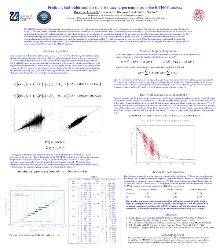
1. The HITEMP database[1] provides molecular spectroscopic parameters for high-temperature modeling of the spectra of molecules in the gas phase. Currently there are 5 molecular species on the database; H2O, CO2, CO, NO, and OH. For H2O, there are now transitions that have rotational quantum numbers up to J = 50 and many transitions where the vibrational quantum numbers and prolate and oblate limit pseudo-quantum numbers (Ka and Kc) are not known. Line-shape parameters are not available for most of these transitions. We have developed a method to determine these line-shape parameters for the 3 most abundant isotopologues of water based on the Semi-empirical approach of Jacquemart et al.[2] and an algorithm that estimates the number of vibrational quanta exchanged in the transition. Thus vibrational dependence of the line-shape parameters, which has been found to be important for H2O[3], is taken into account for many transitions. When the parameters are not available from this new algorithm, average half-widths as a function of J˝ are determined from a polynomial fit of validated calculated data. The results of the new algorithm and the J-averaged half-widths are compared with the values found on the 2008 version of the HITRAN database Empirical algorithm Considering an isolated rovibrational transition (v1′v2′v3′) f ← (v1v2v3) i, where the vk represent the quantum numbers associated with the normal mode of vibration k and the primes and double primes are, respectively, used for the upper and lower level, and i and f are the rotational quantum numbers of the transition. The line shift , and half-width , are given respectively, by the negative of the imaginary part and by the real part of the diagonal element of the complex relaxation matrix. Expanding the sine and cosine terms in the CRB equations, keeping only the first-order terms, and realizing that the vibrational dependence of the polarizability dominates the vibrational dephasing term, yields approximate expressions for  and  for a transition involving various vibrational states but specific sets i and f of rotational quantum numbers. Modified Empirical algorithm A modified empirical algorithm was developed, which uses the straight line fit to determine the number of quanta involved in the transition from the frequency. Given by where as is the stretching coefficient (0.3) and ab is the bend coefficient (0.07), and Predicting half-widths and line shifts for water vapor transitions on the HITEMP databaseRobert R. Gamachea, Laurence S. Rothmanb, and Iouli E. GordonbaDepartment of Environmental, Earth, and Atmospheric SciencesUniversity of Massachusetts Lowell, and the University of Massachusetts School of Marine Sciences, Lowell, MAb Harvard-Smithsonian Center for Astrophysics, Atomic and Molecular Division, Cambridge, MA where fi is the fraction of stretching or bending and si and bi are the number of stretch and bend quanta exchanged. These values are determined using a weighted average of bend and stretch quanta determined from Table 1 for up to 16 units of 2 quanta exchanged. For the number of quanta exchanged >16 we take fsi = 0.8 and fbi = 0.2 for an even number of quanta exchanged and fsi = 0.75 and fbi = 0.25 for an odd number of quanta exchanged. Half-width averaged as a function of J When J is greater than 20 or there are not enough data to use the semi-empirical algorithm, an estimate of the half-width can be obtained from g averaged as a function of J. Since the HITEMP database goes to J = 50, we need to extrapolate  to this value. To accomplish this, the theoretical calculations were studied to find the structure as a function of J. As J increases, the collisional process goes more and more off resonance. This off-resonance limit can be estimated from the values of the prolate limit states (Ka=J). Using these values as the J = 49 and 50 value, a third-order polynomial fit can be made to the averaged air-broadened half-width as a function of J . This fit is shown in the figure below. The results of the fit give γ = 0.106906 – 6.71226 ×10-1J + 1.53337 ×10-2J2 – 1.17092 ×10-4J3 Polyad structure This suggests that the frequency of the transition can be related to the number of vibrational quanta exchanged in the transition. To test this hypothesis, the 2008 HITRAN database was taken and transitions for the principle isotopologue were read. Taking a 2 quanta exchanged as ½ unit and 1 and 3 quanta exchanged as one unit, a plot of quanta exchanged versus frequency was made. Note, in the above expressions the coefficients for 1 and 3 are the same; thus stretch quanta exchanged can be treated equally. This fact allows the number of quanta exchanges to be related the frequency via Testing the new algorithm The alternative to using the new algorithm is to estimate the half-width from J. To test the two methods, the half-widths were determined by the semi-empirical (SE) routine where the number of vibrational quanta are estimated and by the average values as a function of J. The estimated values are compared to the values in the HITRAN database. The statistics of the comparison of the two methods of estimating the half-widths for the 37 432 principal isotopologue transitions in HITRAN are given below. Table 1 †# lines b+s # lines fraction †# lines b+s # lines fraction total total 1 4006 -1 1 1016 0.254 10 2221 0 5 984 0.443 1 0 2990 0.746 2 4 706 0.318 2 5358 0 1 3906 0.729 4 3 477 0.215 2 0 1452 0.271 6 2 36 0.016 3 3362 -1 2 66 0.020 8 1 14 0.006 1 1 2636 0.784 10 0 4 0.002 3 0 660 0.196 11 798 1 5 393 0.492 4 4209 0 2 2534 0.602 3 4 312 0.391 2 1 1414 0.336 5 3 69 0.086 4 0 261 0.062 7 2 16 0.020 5 1793 -1 3 1 0.001 9 1 8 0.010 1 2 1200 0.669 12 898 0 6 522 0.581 3 1 577 0.322 2 5 141 0.157 5 0 15 0.008 4 4 178 0.198 6 3120 0 3 1990 0.638 6 3 36 0.040 2 2 870 0.279 8 2 15 0.017 4 1 253 0.081 10 1 4 0.004 6 0 7 0.002 12 0 2 0.002 7 2350 -1 4 2 0.001 13 346 1 6 229 0.662 1 3 1517 0.646 3 5 66 0.191 3 2 788 0.335 5 4 26 0.075 5 1 41 0.017 7 3 14 0.040 7 0 2 0.001 9 2 7 0.020 8 2945 0 4 1648 0.560 13 0 4 0.012 2 3 1015 0.345 14 289 0 7 243 0.841 4 2 251 0.085 2 6 15 0.052 6 1 27 0.009 4 5 2 0.007 8 0 4 0.001 6 4 28 0.097 9 1603 1 4 961 0.600 8 3 1 0.003 3 3 519 0.324 15 22 1 7 19 0.864 5 2 79 0.049 5 5 1 0.045 7 1 41 0.026 7 4 2 0.091 9 0 3 0.002 16 72 0 8 72 1.000 † number of quanta exchanged in units of 2 Method Average % Difference Average Deviation Standard Deviation J average -9.42 29.86 51.76 SE 9.01 12.27 17.79 Thus it is clear that the new semi-empirical algorithm yields much better half-widths than the simple J -averaged half-width. The new algorithm is now being used to add half-widths, their temperature dependence, and line shifts to BT2[4] transitions that lack vibrational quantum information. When information is lacking, the half-width is estimated from the J average. References 1. L.S. Rothman, I.E. Gordon, R.J. Barber, H. Dothe, R.R. Gamache, A. Goldman, V.I. Perevalov, S.A. Tashkun, J. Tennyson, J. Quant. Spectrosc. Radiat. Transf., in press (2010). 2. D. Jacquemart, R. Gamache, L.S. Rothman, J. Quant. Spectrosc. Radiat. Transf. 96, 205-239 (2005). 3. R.R. Gamache and J.-M. Hartmann, J. Quant. Spectrosc. Radiat. Transf. 83, 119-147 (2004). 4. R.J. Barber, J. Tennyson, G.J. Harris, R.N. Tolchenov, Mon. Not. R. Astron. Soc. 368, 1087-1094 (2006). Acknowledgement One of the authors, RRG, is pleased to acknowledge support of this research by the National Science Foundation through Grant No. ATM-0803135. Any opinions, findings, and conclusions or recommendations expressed in this material are those of the author(s) and do not necessarily reflect the views of the National Science Foundation. The results of the fit give a = 0.30041×10-3 and b = -0.11189.