Download
1 / 24
240 likes | 247 Views
A technique for calculating missed eigenpairs in nonproportionally damped systems using the modified Sturm sequence property. This method is more effective than existing techniques and requires no iterations.

E N D
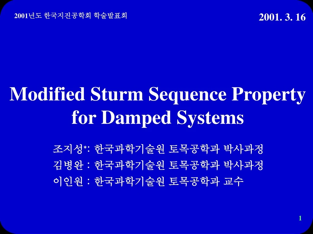
2001. 3. 16 2001년도 한국지진공학회 학술발표회 Modified Sturm Sequence Property for Damped Systems 조지성*: 한국과학기술원 토목공학과 박사과정 김병완 : 한국과학기술원 토목공학과 박사과정 이인원 : 한국과학기술원 토목공학과 교수
Contents 1. Introduction 2. Proposed Method 3. Numerical Example 4. Conclusions
1. Introduction • modal transformation • - dynamic equations of motion modal equations • - transformation matrix : incomplete eigenvector setinexact dynamic response • - checking technique of missed eigenpairs is required.
proportionally damped system • - eigenvalues and eigenvectors : real numbers • - checking technique : sturm sequence property • nonproportionally damped system • (soil-structure interaction problem, structural control • problem, composite structure and so on) • - eigenvalues and eigenvectors : complex numbers • - checking technique : not developed yet. (1) (2)
objective • development of an effective checking technique of • missed eigenpairs applicable to nonproportionally • damped system
2. Proposed Method complex eigenvalue problem (3) linearized form ( ) (4) (5)
characteristic polynomial - given matrix A (6) - characteristic polynomial ,P()=0, eigenvalue (7)
Chen’s algorithm - change of the matrix form (8)
Schur-Cohn Matrix T (10) tij : i-th row, j-th column element of T (11)
Gleyse’s theorem imaginary axis 1 1 -1 Real axis -1 unit disk the number of poles in the unit open disk: (12)
n : degree of the characteristic polynomial P S[k0, k1, k2, ···, kn ]: the number of sign changes in the sequence (ki, i=0, 1, ···, n) (di , i=1, ··· , n): determinant of the leading principal submatrices of order i in the Schur- Cohn matrix T
calculation of di - T=LDLT factorization (13)
the number of zeros in the open disk radius >0 (14) let (15)
3. Numerical Example plane frame structure with lumped dampers L v u L
Given properties Damping Concentrated: 0.3 Rayleigh: = 0.001, = 0.001 Young’s modulus: 1000 Mass density: 1.0 Cross-sectional inertia: 1.0 Cross-sectional area: 1.0 Span length: 6.0 System data Number of elements: 12 Number of nodes: 14 Number of DOF: 18
Mode No. Eigenvalues Radius Real Imaginary 1 -1.137 -46.219 46.233 2 -1.137 +46.219 46.233 3 -1.137 -46.219 46.233 4 -1.137 +46.219 46.233 5 -1.373 -51.133 51.152 6 -1.373 +51.133 51.152 7 -1.373 -51.133 51.152 8 -1.373 +51.133 51.152 9 -3.390 -81.078 81.149 10 -3.390 +81.078 81.149 calculated eigenvalues
Mode No. Eigenvalues Radius Real Imaginary 11 -3.390 -81.078 81.149 12 -3.390 +81.078 81.149 13 -3.941 -87.477 87.566 14 -3.941 +87.477 87.566 15 -3.941 -87.477 87.566 16 -3.941 +87.477 87.566 17 -8.164 -127.439 127.701 18 -8.164 +127.439 127.701 19 -8.164 -127.439 127.701 20 -8.164 +127.439 127.701
Mode No. Eigenvalues Radius Real Imaginary 21 -10.263 -142.837 143.205 22 -10.263 +142.837 143.205 23 -10.263 -142.837 143.205 24 -10.263 +142.837 143.205 25 -14.862 -171.730 172.372 26 -14.862 +171.730 172.372 27 -14.862 -171.730 172.372 28 -14.862 +171.730 172.372 29 -20.537 -201.625 202.668 30 -20.537 +201.625 202.668
Mode No. Eigenvalues Radius Real Imaginary 31 -20.537 -201.625 202.668 32 -20.537 +201.625 202.668 33 -23.770 -216.733 218.033 34 -23.770 +216.733 218.033 35 -23.770 -216.733 218.033 36 -23.770 +216.733 218.033
1 2 3 4 5 6 7 8 9 10 [ + - + - + - + - + - + - + - + - - + - - - + + - - + - - - - + - - + + + +] S 11 12 13 14 15 16 17 18 19 20 21 22 23 24 = 36-24 = 12 O.K
[ + + + + + + + + + + + + + + + + + + + + + + + + + + + + + - + - - - + + +] S 1 2 3 4 = 36- 4 = 32 O.K
[ + + + + + + + + + + + + + + + + + + + + + + + + + + + + + + + + + + + + +] S = 36- 0 = 36 O.K
4. Conclusions • A technique of calculating the number of eigenvalues inside an open disk of arbitrary radius was given. • Comparing to the recently technique by Jung, the proposed method needs no iterations, so more effective than that technique.