Download
1 / 22
220 likes | 227 Views
Hadronic interactions in the SiW ECAL (with the 2008 data). Philippe Doublet, Michele Faucci-Giannelli, Roman Pöschl, François Richard for the CALICE Collaboration. Introduction. 2008 FNAL data used Pions of 2, 4, 6, 8 and 10 GeV Cuts on scintillator and Cherekov counters The SiW ECAL

E N D
Hadronic interactions in the SiW ECAL (with the 2008 data) Philippe Doublet, Michele Faucci-Giannelli, Roman Pöschl, François Richard for the CALICE Collaboration Philippe Doublet (LAL)
Introduction • 2008 FNAL data used • Pions of 2, 4, 6, 8 and 10 GeV • Cuts on scintillator and Cherekov counters • The SiW ECAL • ~1I: more than half of the hadrons interact • 1x1 cm² pixels:tracking possibilities • 30 layers with 3 different W depths 9 Si wafers
Procedure • Follow the MIP track • Find the interaction layer • Distinguish the types of interactions At low energies, finding the interaction and its type requires energy deposition and high granularity
Finding an interaction • Looking at the energy profile in the ECAL • For « strong » interactions • For interactions at smaller energies • Plus classification E(MIPs) Ecut layer E(MIPs) Ecut (fails) Fcut layer
First type: « FireBall » • For inelastic scattering • High energy deposition at rather high energies (Ecut) 10 GeV here • Or relative energy increase at smaller energies (Fcut)2 GeV here X layer Y layer Near the track
E(MIPs) layer Second type: « Pointlike » • For spallation reaction • Local relatively large energy deposition Y layer Pointlike interaction: πp scattering Localised energy deposition +
New type introduced: « Scattered » • Other non interacting events contain two kind of events • Type « Scattered »:pion scattering using the extrapolated incoming MIP and last outgoing hit 2 cells away or more Interesting for Pflow ! • Type « MIP » X layer Y 5 cm ! layer
Optimisation of the cuts (using MC) 8 GeV 3 parameters used: • Standard deviation of the distribution« layer found – true » • Interaction fraction = events found / events with an interaction • Purity with non interacting events = events with no interaction found / events with no interaction • Compromise between those 3 and comparison with David’s method
After optimisation • We care about the interactions found within +/- 1 layer (+/- 2 layers) w.r.t. the interaction layer in the MC +/- 1 layer +/- 2 David +/- 2 David Ward’s results: Ecut criteria made a bit more complex: 3 out of 4 layers must satisfy cut
Rates of interaction from 2 to 10 GeV: data vs MC (5 lists) 2 GeV 4 GeV 6 GeV 10 GeV 8 GeV
Mean shower radius • Transverse size is calculated from the interaction layer (the first for non interacting events):
All events with different energies 2 GeV 4 GeV 6 GeV Reference physics list: QGSP_BERT Very good agreement. 2 GeV starts to have a very different behaviour from other energies. 8 GeV 10 GeV
Classification at 8 GeV « Scattered » « MIP » « FireBall » « Pointlike »
Classification at 2 GeV « Scattered » « MIP » « FireBall » « Pointlike »
Longitudinal profiles • Longitudinal profiles are drawn with 60 layers equivalent to those in the first stack (i.e. one layer in stack 2 is divided in 2 layers and one layer in stack 3 is divided in 3 layers) • Layer 0 is the interaction layer (set to 0 for non interacting events) • The energy deposited in the layer is decomposed in the MC between various secondary particles’ contributions
All events at different energies QGSP_BERT Energies overestimated 2 GeV 4 GeV 6 GeV 8 GeV 10 GeV
FireBall at 8 GeV for different lists QGSP_BERT FTFP_BERT QGSP_BIC LHEP QGS_BIC Good agreement
FireBall at 2 GeV for different lists QGSP_BERT FTFP_BERT Good agreement QGSP_BIC LHEP QGS_BIC
Pointlike at 2 GeV for different lists QGSP_BERT FTFP_BERT Mainly protons Spallation QGSP_BIC LHEP QGS_BIC Mainly nuclear fragments (deuterium, …)
« MIP » and « Scattered » profiles QGSP_BERT 2 GeV 2 GeV Show inefficiencies per layer Excess of EM component 8 GeV 8 GeV
Conclusion • We combine energyandhigh granularity to classify hadronic interactions and even see them clearly • The mean shower radii agree very well • The longitudinal profiles show differencies between physics lists • 4 types of interaction allow to separate clearly the profiles and show points of improvement for the lists • Showers of types « FireBall » and « Pointlike » to be investigated • Type « Scattered » very promising for particle flow studies (to be improved – ex: angular distribution studies) • Results stable obtained with official releases
Pointlike at 8 GeV for different lists QGSP_BERT FTFP_BERT QGSP_BIC LHEP QGS_BIC