Download
1 / 16
160 likes | 174 Views
Lec 3. System Modeling. Transfer Function Model Model of Mechanical Systems Model of Electrical Systems Model of Electromechanical Systems. TexPoint fonts used in EMF. Read the TexPoint manual before you delete this box.: A A A. Transfer Functions of LTI Systems.

E N D
Lec 3. System Modeling • Transfer Function Model • Model of Mechanical Systems • Model of Electrical Systems • Model of Electromechanical Systems TexPoint fonts used in EMF. Read the TexPoint manual before you delete this box.: AAA
Transfer Functions of LTI Systems Output of a linear time-invariant (LTI) system is given by where is the impulse response, output under input u(t)=(t) Take the Laplace transform: is called the transfer function
LTI Systems Given by Differential Equations Common LTI system models for practical systems: Assuming zero initial condition, transfer function model is (in general)
(Rational) Transfer Functions • n-th order system • Zeros: roots of , • Poles: roots of , Pole zero plot:
Standard Forms of Rational Transfer Functions Basic form: • Matlab commands: tf, tfdata Factored (or product) form: • Matlab commands: zpk, zpkdata Sum form (assume poles are distinct): If all poles are distinct p1,…,pn are the poles, r1,…,rn are the corresponding residues
Example: Car Suspension Model (body) m2 shock absorber (wheel) m1 Input: road altitude r(t) Output: car body height y(t) road surface
Suspension System Model Differential equation model:
Translational Mechanical System Models • Identify all independent components of the system • For each component, do a force analysis (all forces acting on it) • Apply Newton’s Second Law to obtain an ODE, and take the Laplace transform of it • Combine the equations to eliminate internal variables • Write the transfer function from input to output
Rotational Mechanical Systems: Satellite gas jet Suppose that the antenna of the satellite needs to point to the earth Ignore the translational motions of the satellite Input: A force F generated by the release of reaction jet Output: orientation of the satellite given by the angle
Satellite Model Torque: In general gas jet Newton’s Second Law:
Model of Electrical Systems Basic components resistor inductor capacitor
Impedance Basic components resistor inductor capacitor
Electromechanical System: DC Motor Armature resistance Torque T Basic motor properties: Torque proportional to current: Motor voltage proportional to shaft angular velocity: Friction B Input: voltage source e(t) Output: shaft angular position q(t) Newton law: Basic circuit properties (KVL):
Nonlinear System: Pendulum pendulum Input: external force F Output: angle Dynamic equation from Newton’s law