Download
1 / 39
390 likes | 401 Views
Granular Simulation. Junbang Liang. Contents. Introduction Motivation Granular Modeling Particle-based method Fluid-based method Others. Introduction. Motivation. Granular Modeling - Properties. Different from solid: Flowing freely if in low coherence

E N D
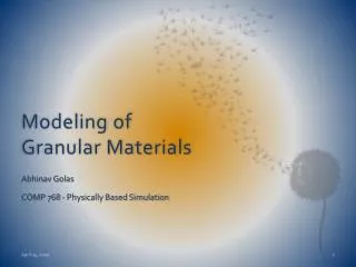
Granular Simulation Junbang Liang
Contents • Introduction • Motivation • Granular Modeling • Particle-based method • Fluid-based method • Others
Granular Modeling - Properties • Different from solid: • Flowing freely if in low coherence • Forms different shapes if in high coherence • Large number of small separate particles • Different from fluid: • Piling, maximum rest angle • Pressure is independent to depth • Frictional and contact forces between particles
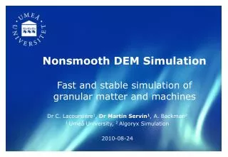
Granular Modeling - Methods • Particle-based method • Treat each one of the grain as a rigid body • Memory and computation intensive • Fluid-based method • Treat the grain as a whole • Modify fluid simulation equations • Others • Height field • Deformable body
Particle-based methods • Luciani, Annie, ArashHabibi, and Emmanuel Manzotti. "A multi-scale physical model of granular materials." Graphics interface'95. 1995. • A grain is represented as a spring-mass system. • External forces are formulated as springs as well.
Spring-Mass System • Dynamics: Classic ODE solver • k: stiffness coefficient, z: damping coefficient • d12: string length, d0: string length at rest • x, y: displacement • FL is used inside the particle, FNL is used between particles.
Spring-Mass System • Inside the grain: linear, stiff strings • Between sand particles: nonlinear strings • Easy to implement • Only in small scale; time step is limited
Particle-based methods(cont.) • Bell, Nathan, Yizhou Yu, and Peter J. Mucha. "Particle-based simulation of granular materials." Proceedings of the 2005 ACM SIGGRAPH/Eurographics symposium on Computer animation. ACM, 2005. • Using sphere as the primitive, defining contact forces on collision. • Model rigid bodies and grains as a collection of spheres.
Rigid Sphere Dynamics • Particle overlap: , Normal direction: • Relative velocity: , , • Normal forces: where • Shear forces: • Resolving static friction:using non-spherical particles
Rigid Sphere Dynamics • Efficient if given fast collision detection algorithm • The accuracy of rigid bodies are parameterized • Particles are independent: neglects the cohesive forces between particles
Fluid-based method • Model granular as a incompressible continuum. • Independent of the actual number of particles. • Follows the rule of simulating fluid. Flowing can be achieved naturally. • Additional check to approximate friction and contact forces.
Navier-Stokes Equation • Reynolds transport theorem: conservation of any physical property within any control volume. • Change of in equals to the amount of that flows out of , plus the speed of generating from sources in . • dV: infinitesimal Volume, u=(t): Flow velocity, n: Normal vector of the surface, A: Surface area, s: Property source/sink in . • Divergence theorem, Leibniz’s rule: • can be mass() or momentum()
Navier-Stokes Equation(cont.) • Reynolds transport theorem: • Conservation of mass • , • At point x, the increase of density plus the amount of the divergence (dissipation) of density at that point equals to 0. • Conservation of momentum • At point x, the increase of momentum plus the amount of the divergence of momentum , where denotes the momentum at dimension k, equals to the increase of momentum from the source at that point.
Navier-Stokes Equation(cont.) • Dyad: • Divergence of a matrix: • Ai is the ith column of A
Navier-Stokes Equation(cont.) • Split each term above: • => • Rearrange: • Conservation of mass: • , where
Navier-Stokes Equation(cont.) • S is the source of momentum, that is, forces. • : Stress tensor, : External forces, e.g. gravity. • p: Pressure, : Shear stress tensor. • , • is depending on the kind of fluid, e.g., for incompressible Newtonian fluid, . • is computed so that conservation of mass is maintained.
Lagrangian/Eulerian reference system • Grid representation: Particle representation: • The left side is the property gradient of this specific particle, while is originally defined in Eulerian perspective. • could be any physical properties: temperature, density, or flow velocity
Simulation Method • , • Particle based • Represent the continuum with a set of particles • Each particle carries physical properties, e.g., mass, density and velocity • Using interpolation kernel to express the continuum • Examples: Smoothed Particle Hydrodynamic. • Grid based • Hybrid approach
Simulation Method • , • Particle based • Grid based • Represent the continuum with a number of fixed grid points • Each grid point carries physical properties, e.g., mass, density and velocity • The partial differentiation is approximated as finite difference between adjacent grid points • Hybrid approach
Pros and Cons • , • Particle based • Automatically guarantees conservation of mass • Difficult to deal with partial differential equations • Grid based • Partial difference can be expressed easily • More computation to keep conservation
Simulation method • Hybrid approach: Particle-In-Cell (PIC), FLuid Implicit Particle (FLIP), Material Point Method (MPM). • Particles are good for moving (kinematic), grids are good for solving PDE (dynamic). • FLIP updates velocity using increments instead of direct interpolation. • MPM uses particle to carry all of the physical property including stress and forces.
Splitting • Example equation: • Explicit Euler: • General form: • Hybrid method: , , q=u • f=- • g={, s.t.} • F is done in Lagrangian frame (particles), G is done in Eulerian frame (grid).
Fluid-based method • Drucker, Daniel Charles, and William Prager. "Soil mechanics and plastic analysis or limit design." Quarterly of applied mathematics 10.2 (1952): 157-165. • : shear stress, : friction coefficient, : pressure, : cohesion • Drucker-Prager yield condition
First trial(2005) • Zhu, Yongning, and Robert Bridson. "Animating sand as a fluid." ACM Transactions on Graphics (TOG). Vol. 24. No. 3. ACM, 2005. • Assumptions: • Sand pressure is the same as incompressible fluid. • If flowing, frictional stress is defined as: • : Repost (rest) angle, D: strain rate, u: velocity • Using Drucker-Prager yield condition to determine whether it is flowing or not
First trial(2005) • Grid length , shear velocity , grid mass • Force to stop shearing in one time step: • Shear stress: • Classify grids with rigid and deforming ones.
First trial(2005) • Do advection on particles and transfer to grid • Add gravity and solve pressure to make it incompressible. • Calculate using current velocity field. • Check if satisfies the yield condition, where . • If not, the grid is rigid; otherwise using to update velocity. • Find all connected rigid grids and solve it as a rigid body. • Transfer to particles.
Improvements(2010) • Narain, Rahul, AbhinavGolas, and Ming C. Lin. "Free-flowing granular materials with two-way solid coupling." ACM Transactions on Graphics (TOG)29.6 (2010): 173. • Main observation: Sand cannot be compressed, but can be splashed out. . Internal pressure will be 0 if . • Define density fraction: • Conservation of mass and momentum: • => • Density fraction at time n+1:
Solving pressure • Goal: calculate p, so that: • Extra conditions: Internal pressure will be 0 if . • Linear complementary problem: • : Density must not exceed maximum value • : Pressure works when flow is no more compressible • : Pressure should be non-negative
Solving pressure • Gradient matrix: • D is the matrix that maps the field of to the field of • , • From definition to matrix formulation: • => where
Solving pressure • Asdf • Karush–Kuhn–Tucker conditions: • , where • , which means • , which means
Solving friction • Drucker-Prager yield condition: • Linearization: • The principle of maximum plastic dissipation [Simo and Hughes 1998] • Maximize the dissipation of kinetic energy => minimize kinetic energy • where with • : density, : intermediate velocity,
Solving friction • Linearization: • Gradient matrix:
Overall process • For each time step: • Accumulate density and velocity onto grid. • Repeat until convergence or maximum iterations: • Compute frictions by minimizing E(s) for fixed p. • Compute pressure by minimizing f(p) for fixed s. • Find intermediate velocity v ̃. • Update particles: • (a) Update velocities using FLIP. • (b) Move particles through the velocity field v ̃.
Details and Extensions • Boundary conditions • Not penetrating the wall • Interaction with solid bodies • Define the volume fraction • Add the affect to , and • Multiple Material with different density • Modify the calculation of • Rendering • [Brackbill and Ruppel 1986; Zhu and Bridson 2005]
Further refinement • Extends Zhu’s work to SPH and adds interactions with fluids(2009) • Lenaerts, Toon, and Philip Dutré. "Mixing fluids and granular materials." Computer Graphics Forum. Vol. 28. No. 2. Blackwell Publishing Ltd, 2009. • Extends Narain’s approach to SPH and add cohesion(2011) • Alduán, Iván, and Miguel A. Otaduy. "SPH granular flow with friction and cohesion." Proceedings of the 2011 ACM SIGGRAPH/Eurographics Symposium on Computer Animation. ACM, 2011. • Uses semi-implicit integration on MPM without linearization(2016) • Daviet, Gilles, and Florence Bertails-Descoubes. "A Semi-Implicit Material Point Method for the Continuum Simulation of Granular Materials." ACM Transactions on Graphics 35.4 (2016): 13.
Other approaches • Uses height field to simulate tracks and footprints on sand(1999) • Sumner, Robert W., James F. O'Brien, and Jessica K. Hodgins. "Animating sand, mud, and snow." Computer Graphics Forum. Vol. 18. No. 1. Blackwell Publishers Ltd, 1999. • Uses deformable body rather than rigid particles on MPM to simulate snow(2013)(Frozen) • Stomakhin, Alexey, et al. "A material point method for snow simulation." ACM Transactions on Graphics (TOG) 32.4 (2013): 102. • Uses similar method to simulate sand(2016) • Klár, Gergely, et al. "Drucker-pragerelastoplasticity for sand animation." ACM Transactions on Graphics (TOG) 35.4 (2016): 103.
References • Luciani, Annie, ArashHabibi, and Emmanuel Manzotti. "A multi-scale physical model of granular materials." Graphics interface'95. 1995. • Bell, Nathan, Yizhou Yu, and Peter J. Mucha. "Particle-based simulation of granular materials." Proceedings of the 2005 ACM SIGGRAPH/Eurographics symposium on Computer animation. ACM, 2005. • Drucker, Daniel Charles, and William Prager. "Soil mechanics and plastic analysis or limit design." Quarterly of applied mathematics 10.2 (1952): 157-165. • Zhu, Yongning, and Robert Bridson. "Animating sand as a fluid." ACM Transactions on Graphics (TOG). Vol. 24. No. 3. ACM, 2005. • Narain, Rahul, AbhinavGolas, and Ming C. Lin. "Free-flowing granular materials with two-way solid coupling." ACM Transactions on Graphics (TOG)29.6 (2010): 173. • Lenaerts, Toon, and Philip Dutré. "Mixing fluids and granular materials." Computer Graphics Forum. Vol. 28. No. 2. Blackwell Publishing Ltd, 2009. • Alduán, Iván, and Miguel A. Otaduy. "SPH granular flow with friction and cohesion." Proceedings of the 2011 ACM SIGGRAPH/Eurographics Symposium on Computer Animation. ACM, 2011. • Daviet, Gilles, and Florence Bertails-Descoubes. "A Semi-Implicit Material Point Method for the Continuum Simulation of Granular Materials." ACM Transactions on Graphics 35.4 (2016): 13. • Sumner, Robert W., James F. O'Brien, and Jessica K. Hodgins. "Animating sand, mud, and snow." Computer Graphics Forum. Vol. 18. No. 1. Blackwell Publishers Ltd, 1999. • Stomakhin, Alexey, et al. "A material point method for snow simulation." ACM Transactions on Graphics (TOG) 32.4 (2013): 102. • Klár, Gergely, et al. "Drucker-pragerelastoplasticity for sand animation." ACM Transactions on Graphics (TOG) 35.4 (2016): 103.