Download
1 / 59
630 likes | 904 Views
Chapter 4 The Simplex Algorithm PART 1. Ass oc . Prof. Dr. Arslan M. ÖRNEK. Example 1: Leather Limited. Leather Limited manufactures two types of leather belts: the deluxe model and the regular model. Each type requires 1 square yard of leather.

E N D
Chapter 4The Simplex AlgorithmPART 1 Assoc. Prof. Dr. Arslan M. ÖRNEK
Example 1: Leather Limited • Leather Limited manufactures two types of leather belts: the deluxe model and the regular model. • Each type requires 1 square yard of leather. • A regular belt requires 1 hour of skilled labor and a deluxe belt requires 2 hours of skilled labor. • Each week, 40 square yards of leather and 60 hours of skilled labor are available. • Each regular belt contributes $3 profit and each deluxe belt $4. • Write an LP to maximize profit.
Example 1: Solution • The decision variables are: • x1 = number of deluxe belts produced weekly • x2 = number of regular belts produced weekly • The appropriate LP is: max z = 4x1 + 3x2 s.t. x1 + x2≤ 40 (leather constraint) 2x1 +x2 ≤ 60 (labor constraint) x1, x2 ≥ 0
4.1 – How to Convert an LP to Standard Form Before the simplex algorithm can be used to solve an LP, the LP must be converted into a problem where • all the constraints are equations and • all variables are nonnegative. An LP in this form is said to be in standard form. (why?)
To convert a “≤ “ constraint to an equality, • Define for each constraint a slack variablesi (si = slack variable for the ith constraint). A slack variable is the amount of the resource unused in the ith constraint. • Convert constraint i into an equality constraint by adding the slack variable si • Add the sign restriction si ≥ 0 to the model.
4.1 – How to Convert an LP to Standard Form The LP not in standard form is: max z = 4x1 + 3x2 s.t. x1 + x2 ≤ 40 (leather constraint) 2x1 + x2 ≤ 60 (labor constraint) x1, x2 ≥ 0 The same LP in standard form is: max z = 4x1 + 3x2 s.t. x1 + x2 + s1= 40 2x1 + x2 + s2= 60 x1, x2, s1, s2 ≥ 0
To convert the ith “≥” constraint to an equality constraint, • Define an excess variable(sometimes called a surplus variable) ei. • We define ei to be the amount by which ith constraint is oversatisfied. • Subtract the excess variable ei from the ith constraint • Add the sign restriction ei ≥ 0 to the model. • If an LP has both ≤ and ≥ constraints, convert all to equality.
4.1 – How to Convert an LP to Standard Form Consider the formulation below: min z = 50 x1 + 20x2 + 30x3+ 80 x4 s.t. 400x1 + 200x2 + 150 x3 + 500x4 ≥ 500 3x1 + 2x2 ≥ 6 2x1 + 2x2 + 4x3 + 4x4≥ 10 2x1 + 4x2 + x3 + 5x4≥ 8 x1, x2, x3, x4 ≥ 0
4.1 – How to Convert an LP to Standard Form min z = 50 x1 + 20x2 + 30X2 + 80 x4 s.t. 400x1 + 200x2 + 150 x3 + 500x4 ≥ 500 3x1 + 2x2 ≥ 6 2x1 + 2x2 + 4x3 + 4x4≥ 10 2x1 + 4x2 + x3 + 5x4≥ 8 x1, x2, x3, x4 ≥ 0 min z = 50 x1 + 20x2 + 30X2 + 80 x4 s.t. 400x1 + 200x2 + 150 x3 + 500x4 – e1 = 500 3x1 + 2x2- e2 = 6 2x1 + 2x2 + 4x3 + 4x4- e3= 10 2x1 + 4x2 + x3 + 5x4- e4= 8 xi, ei > 0 (i = 1,2,3,4)
4.1 – How to Convert an LP to Standard Form Nonstandard Form Standard Form max z = 20x1 + 15x2 s.t. x1+ s1 = 100 x2 + s2= 100 50x1 + 35x2+ s3= 6000 20x1 + 15x2- e4= 2000 x1, x2, s1, s2, s3, e4 > 0 max z = 20x1 + 15x2 s.t. x1≤ 100 x2≤ 100 50x1 + 35x2≤ 6000 20x1 + 15x2≥ 2000 x1, x2 > 0
4.2 – Preview of the Simplex Algorithm Suppose an LP with m constraints and n variables has been converted into standard form. The form of such an LP is: max ( or min) z = c1x1 + c2x2 + … +cnxn s.t. a11x1 + a12x2 + … + a1nxn =b1 a21x1 + a22x2 + … + a2nxn =b2 . . . . . . am1x1 + am2x2 + … + amnxn =bm xi ≥ 0 ( i = 1,2, …, n)
4.2 – Preview of the Simplex Algorithm If we define: The constraints may be written as a system of equations Ax = b. Consider a system Ax = b of m linear equations in n variables (where n ≥ m). (How many solutions are there for such a system?) A basic solutionto Ax = b is obtained by setting n – mvariables equal to 0 and solving for the remaining m variables. This assumes that setting the n – m variables (Nonbasic variables - NBV) equal to 0 yields a unique value for the remaining m variables, or equivalently, the columns for the remaining m variables are linearly independent.
4.2 – Preview of the Simplex Algorithm x1 + x2 = 3 - x2 + x3 = -1 Different choices of nonbasic variables will lead to different basic solutions. The number of nonbasic variables = 3 – 2 = 1. If NBV = {x3} , then BV = {x1, x2}. Thus, x1 = 2, x2 = 1, and x3 = 0 is a basic solution. x1 + x2 = 3 - x2 + 0 = -1 If NBV = {x1} and BV = {x2, x3}, the basic solution becomes x1 = 0, x2 = 3, and x3 = 2. If NBV = {x2} and BV = {x1, x3}, the basic solution becomes x1 = 3, x2 = 0, and x3 = -1.
4.2 – Preview of the Simplex Algorithm Some sets of m variables do not yield a basic solution. If NBV = {x3} and BV = {x1, x2} the corresponding basic solution would be: x1 + 2x2 + x3 = 1 2x1 + 4x2 + x3 = 3 x1 + 2x2 = 1 2x1 + 4x2 = 3 Since this system has no solution, there is no basic solution corresponding to BV = {x1, x2}. WHY?
4.2 – Preview of the Simplex Algorithm Any basic solution in which all variables are nonnegative is called a basic feasible solution (or bfs). x1 = 2, x2 = 1, x3 = 0 and x1 = 0, x2 = 3, x3 = 2 are basic feasible solutions, x1 = 3, x2 = 0, x3 = -1 is not a bfs (because x3 < 0). bfs’s are important: Theorem 1The feasible region for any linear programming problem is a convex set. Also, if an LP has an optimal solution, there must be an extreme point of the feasible region that is optimal. Theorem 2For any LP, there is a unique extreme point of the LP’s feasible region corresponding to each basic feasible solution. Also, there is at least one bfs corresponding to each extreme point in the feasible region.
4.2 – Preview of the Simplex Algorithm The relationship between extreme points and basic feasible solutions in the Leather Limited problem. max z = 4x1 + 3x2 s.t. x1 + x2 + s1= 40 2x1 + x2 + s2 = 60 x1, x2, s1, s2 ≥ 0 The extreme points of the feasible region are B, C, E, and F. How many are there basic solutions? n=4, m=2
4.2 – Preview of the Simplex Algorithm The table above shows the correspondence between the basic feasible solutions to the LP and the extreme points of the feasible region. The basic feasible solutions to the standard form of the LP correspond in a natural fashion to the LP’s extreme points. BFS = Corner Point Feasible Solution (CFP)
Adjacent Basic Feasible Solutions Theorem 3If an LP has an optimal solution, then it has an optimal bfs. For example, in the Leather Limited LP, the bfs corresponding to point E is adjacent to the bfs corresponding to point C. These points share (m – 1 = 2 - 1 = 1) one basic variable, x1. Points E (BV = {x1,x2}) and F (BV = {s1,s2}) are not adjacent since they share no basic variables. Intuitively, two basic feasible solutions are adjacent if they both lie on the same edge of the boundary of the feasible region. DefinitionFor any LP with m constraints, two basic feasible solutions are said to be adjacent if their sets of basic variables have m – 1 basic variables in common.
Basic, Nonbasic Solutions and the Basis • In an LP, number of variables (n) > number of equations (m) • The difference is the degrees of freedom of the system • Set some variables (n-m) to an arbitrary value (simplex uses 0) • These variables (set to 0) are called nonbasic variables • The rest can be found by solving the remaining system: basis • The basis: the set of basic variables • If all basic variables are ≥ 0, we have a BFS
Basic and Basic Feasible Solutions X2 Standard Form Maximize Z = 3x1+ 5x2 subject to x1+s1= 4 2x2+s2= 12 3x1+ 2x2+s3= 18 x1,x2, s1, s2, s3 ≥ 0 (0,9,4,-6,0) (0,6,4,0,6) (2,6,2,0,0) (4,6,0,0,-6) • Basic solution (corners) • Basic infeasible solution (4,6) • Basic feasible solution (BFS) (4,3) • Nonbasic feasible solution (2,3,2,6,6) (4,3,0,6,0) (0,2,4,8,14) (0,0,4,12,18) (4,0,0,12,6) (6,0,-2,12,0) X1
Adjacent Basic Feasible Solutions General description of the simplex algorithm solving an LP in a maximization problem: Step 1Find a bfs to the LP. We will call this bfs the initial bfs. In general, the most recent bfs will be called the current bfs. Step 2 Determine if the current bfs is an optimal solution to the LP. If it is not, find an adjacent bfs that has a larger z-value. Step 3Return to Step 2, using the new bfs as the current bfs.
4.3 – The Simplex Algorithm (max LPs) The Simplex Algorithm Procedure for maximization LPs Step 1 Convert the LP to standard form Step 2 Obtain a bfs (if possible) from the standard form Step 3 Determine whether the current bfs is optimal Step 4 If the current bfs is not optimal, determine which nonbasic variable should become a basic variable and which basic variable should become a nonbasic variable to find a bfs with a better objective function value. Step 5 Use ero’s to find a new bfs with a better objective function value. Go back to Step 3. In performing the simplex algorithm, write the objective function in the form: z – c1x1 – c2x2 - … - cnxn = 0 We call this format the row 0 version of the objective function (row 0 for short).
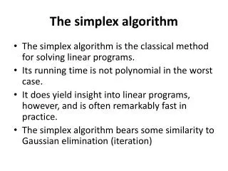
4.3 – The Simplex Algorithm (max LPs) • Simplex method is an algebraic procedure • However, its underlying concepts are geometric • Understanding these geometric concepts helps before going into their algebraic equivalents
Optimality test Consider any LP problem that possesses at least one optimal solution. If a BFS(corner point feasible solution - CFP) has no adjacentBFS that is better (as measured by Z), then it must be an optimal solution. • (2,6) must be optimal since Z=36 is greater than Z=30 for (0,6) and Z=27 for (4,3). • This is the optimality test used by Simplex.
The Simplex Method in a Nutshell Initialization (Find initial CPF solution) Is the current CPF solution optimal? Yes Stop No Move to a better adjacent CPF solution
Algebra of the Simplex MethodInitialization Maximize Z = 3x1+ 5x2 subject to x1+s1= 4 2x2+s2= 12 3x1+ 2x2+s3 = 18 x1,x2, s1, s2, s3 ≥ 0 • Find an initial basic feasible solution • If possible, use the origin as the initial BFS • Equivalent to:Choose original variables to be nonbasic (xi=0, i=1,…n) and let the slack variables be basic (sj=bj, j=1,…m))
Algebra of the Simplex MethodOptimality Test Maximize Z = 3x1+ 5x2 subject to x1+s1= 4 2x2+s2= 12 3x1+ 2x2+s3 = 18 x1,x2, s1, s2, s3 ≥ 0 • Is any adjacent BFS better than the current one? • Rewrite Z in terms of nonbasic variables and investigate rate of improvement • Current nonbasic variables:x1,x2 • Corresponding Z= 0 • Optimal? No. If I increase the value of one of the nonbasic variables from 0 to a positive value, the objective function will increase.
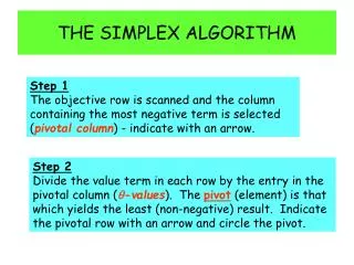
Algebra of the Simplex MethodStep 1 of Iteration 1: Direction of Movement Maximize Z = 3x1+ 5x2 subject to x1+s1= 4 2x2+s2= 12 3x1+ 2x2+s3 = 18 x1,x2, s1, s2, s3 ≥ 0 • Which edge to move on? • Determine the direction of movement by selecting the entering variable (variable ‘entering’ the basis) • Choose the direction of steepest ascent (increase, since maximization) • x1: Rate of improvement in Z =3 • x2: Rate of improvement in Z =5 • Entering basic variable = x2(pivot column)
Algebra of the Simplex MethodStep 2 of Iteration 1: Where to Stop Maximize Z = 3x1+ 5x2 subject to x1+s1= 4 (1) 2x2+s2= 12 (2) 3x1+ 2x2+s3 = 18 (3) x1,x2, s1, s2, s3 ≥ 0 • How far can we go? • Determine where to stop by selecting the leaving variable(variable ‘leaving’ the basis) • Increasing the value of x2 decreases the value of basic variables. • The minimum ratio test • Constraint (1):x1≤4 no bound on x2(s1= 4 - x1≥ 0) • Constraint (2):2x2+s2= 12 x2can be increased up to 6 before s2= 0. Min. Ratio • Constraint (3):3x1+2x2+s3= 18 x2can be increased up to 9 before s3= 0. • Leaving basic variable = s2(pivot row)
Algebra of the Simplex MethodStep 3 of Iteration 1: Solving for the New BF Solution Z - 3x1- 5x2 = 0 (0) x1 +s1 = 4 (1) 2x2 +s2 = 12 (2) 3x1+ 2x2 +s3 = 18 (3) Z - 3x1+ + 5/2 s2 = 30 (0) x1 +s1 = 4 (1) x2 + 1/2 s2 = 6 (2) 3x1 - s2 + s3 = 6 (3) • Convert the system of equations to a more proper form for the new BFS • Elementary row operations: Gaussian elimination • Eliminate the entering basic variable (x2) from all but constraint 2 (pivot row) • Since x1=0 and s2=0 we obtain (x1,x2,s1,s2,s3)= (0,6,4,0,6)
Algebra of the Simplex MethodOptimality Test Z - 3x1+ + 5/2 s2 = 30 (0) x1 +s1 = 4 (1) x2 + 1/2 s2 = 6 (2) 3x1 - s2 + s3 = 6 (3) • Is any adjacent BFS better than the current one? • Current nonbasic variables:x1, s2 • Corresponding Z= 30 • Optimal? No (increasing x1increases Z value)
Algebra of the Simplex MethodStep 1 of Iteration 2: Direction of Movement Z - 3x1+ + 5/2 s2 = 30 (0) x1 +s1 = 4 (1) x2 + 1/2 s2 = 6 (2) 3x1 - s2 + s3 = 6 (3) • Which edge to move on? • Determine the direction of movement by selecting the entering variable (variable ‘entering’ the basis) • Choose the direction of steepest ascent • x1: Rate of improvement in Z = 3 • s2: Rate of improvement in Z = - 5/2 • Entering basic variable = x1
Algebra of the Simplex MethodStep 2 of Iteration 2: Where to Stop Z - 3x1+ + 5/2 s2 = 30 (0) x1 +s1 = 4 (1) x2 + 1/2 s2 = 6 (2) 3x1 - s2 + s3 = 6 (3) • How far can we go? • Determine where to stop by selecting the leaving variable (variable ‘leaving’ the basis) • Increasing the value of x1 decreases the value of basic variables • The minimum ratio test • Constraint (1):x1 ≤ 4 • Constraint (2): no upper bound on x1 • Constraint (3):x1 ≤ 6/3= 2 • Leaving basic variable = s3
Algebra of the Simplex MethodStep 3 of Iteration 2: Solving for the New BF Solution Z - 3x1+ + 5/2 s2 = 30 (0) x1 +s1 = 4 (1) x2 + 1/2 s2 = 6 (2) 3x1 - s2 + s3 = 6 (3) Z + 3/2 s2 + s3 = 36 (0) +s1 + 1/3 s2 - 1/3 s3 = 2 (1) x2 + 1/2 s2 = 6 (2) x1 - 1/3 s2 + 1/3 s3 = 2 (3) • Convert the system of equations to a more proper form for the new BFS • Elementary algebraic operations: Gaussian elimination • Eliminate the entering basic variable (x1) from all but its equation • The next BFS: (x1,x2,s1,s2,s3)= (2,6,2,0,0)
Algebra of the Simplex MethodOptimality Test Z + 3/2 s2 + s3 = 36 (0) +s1 + 1/3 s2 - 1/3 s3 = 2 (1) x2 + 1/2 s2= 6 (2) x1 - 1/3 s2 + 1/3 s3 = 2 (3) • Is any adjacent BFS better than the current one? • Current nonbasic variables: s2, s3 • Corresponding Z= 36 • Optimal?yes
4.3 – The Simplex Algorithm (max LPs) The Dakota Furniture company manufactures desk, tables, and chairs. The manufacturer of each type of furniture requires lumber and two types of skilled labor: finishing and carpentry. The amount of each resource needed to make each type of furniture is given in the table below.
4.3 – The Simplex Algorithm (max LPs) At present, 48 board feet of lumber, 20 finishing hours, 8 carpentry hours are available. A desk sells for $60, a table for $30, and a chair for $ 20. Dakota believes that demand for desks and chairs is unlimited, but at most 5 tables can be sold. Since the available resources have already been purchased, Dakota wants to maximize total revenue.
4.3 – The Simplex Algorithm (max LPs) Define: x1 = number of desks produced x2 = number of tables produced x3 = number of chairs produced. The LP is: max z = 60x1 + 30x2 + 20x3 s.t. 8x1 + 6x2 + x3 ≤ 48 (lumber constraint) 4x1 + 2x2 + 1.5x3 ≤ 20 (finishing constraint) 2x1 + 1.5x2 + 0.5x3 ≤ 8 (carpentry constraint) x2≤ 5 (table demand constraint) x1, x2, x3 ≥ 0
4.3 – The Simplex Algorithm (max LPs) Step 1 - Convert the LP to Standard Form If we set x1 = x2 = x3 = 0, we can solve for the values s1, s2, s3, s4. Thus, BV = {s1, s2, s3, s4} and NBV = {x1, x2, x3 }. Since each constraint is then in canonical form (BVs have a coefficient = 1 in one row and zeros in all other rows) with a nonnegative rhs, a bfs can be obtained by inspection.
4.3 – The Simplex Algorithm (max LPs) Step 2 – Obtain a Basic Feasible Solution To perform the simplex algorithm, we need a basic (although not necessarily nonnegative) variable for row 0. Since z appears in row 0 with a coefficient of 1, and z does not appear in any other row, we use z as the basic variable. With this convention, the basic feasible solution for our initial canonical form has: BV = {z, s1, s2, s3, s4} and NBV = {x1, x2, x3 }. For this initial bfs, z = 0, s1= 48, s2= 20, s3 = 8, s4 =5, x1= x2 = x3 = 0. As this example indicates, a slack variable can be used as a basic variable if the rhs of the constraint is nonnegative.
4.3 – The Simplex Algorithm (max LPs) Step 3 – Determine if the Current BFS is Optimal Once we have obtained a bfs, we need to determine whether it is optimal. To do this, we try to determine if there is any way z can be increased by increasing some nonbasic variable from its current value of zero while holding all other nonbasic variables at their current values of zero. Solving for z in row 0 yields: Z = 60x1 + 30x2 + 20x3 BV = {z, s1, s2, s3, s4} and NBV = {x1, x2, x3 }. Increasing any of the nonbasic variables will cause an increase in z. However increasing x1 causes the greatest rate of increase in z. If x1 increases from its current value of zero, it will have to become a basic variable. For this reason, x1 is called the entering variable. Observe x1 has the most negative coefficient in row 0.
4.3 – The Simplex Algorithm (max LPs) Step 4 - Choose the entering variable (in a max problem) as the nonbasic variable with the most negative coefficient in row 0 (ties broken arbitrarily). We desire to make x1 as large as possible but as we do, the current basic variables (s1, s2, s3, s4) will change value. Thus, increasing x1 may cause a basic variable to become negative. RATIO From row 1 we see that s1 = 48 – 8x1. Since s1≥ 0, x1 ≤ 48 / 8 = 6 From row 2, we see that s2 = 20 – 4x1. Since s2≥ 0, x1 ≤ 20 / 4 = 5 From row 3, we see that s3 = 8 – 2x1. Since s3≥ 0, x1 ≤ 8 / 2 =4 From row 4, we see that s4 = 5. For any x1, s4 will always be ≥ 0 This means to keep all the basic variables nonnegative, the largest we can make x1 is min {6, 5, 4} = 4.
4.3 – The Simplex Algorithm (max LPs) The Ratio Test When entering a variable into the basis, compute the ratio: rhs of row / coefficient of entering variable in row for every constraint in which the entering variable has a positive coefficient. The constraint with the smallest ratio is called the winner of theminimum ratio test. The smallest ratio is the largest value of the entering variable that will keep all the current basic variables nonnegative. Make the entering variable x1 a basic variable in row 3 since this row (constraint) was the winner of the ratio test (8/2 =4). Then, s3 will be nonbasic.
4.3 – The Simplex Algorithm (max LPs) To make x1 a basic variable in row 3, we use elementary row operations (EROs) to make x1 have a coefficient of 1 in row 3 and a coefficient of 0 in all other rows. This procedure is called pivoting on row 3; and row 3 is called the pivot row. The final result is that x1 replaces s3 as the basic variable for row 3. The term in the pivot row that involves the entering basic variable is called the pivot term (pivot element). Step 5 - The Gauss-Jordan method using ero’s and simplex tableaus shown on the next slide makes x1 a basic variable.