Homographies , Image Mosaics and Tracking

1. Homographies, Image Mosaics and Tracking Assignment 2

2. Outline • Previously??? • Homography Estimation • Mandatory assignment 2 • Uses of Homographies • Linear texture mapping • Stitching • Perhaps a little on perspective projection • Camera matrix • Camera calibration matrix

3. HOMOGRAPHIES REVISITED

4. Homography matrix (3x3) A special case, planes Observer 2D 2D Image plane (retina, film, canvas) World plane A plane to plane projective transformation

5. Applications of homographies

6. Look at How Individual Features move

7. Some issues • How to estimate H given correspondences? • Number of measurements needed for estimating H

8. Cross product as Matrix Multiplication

9. Homography Estimation How to solve this equation (remember that it the elements in H that needs to be estimated)? 8 degrees of freedom Each pair (x,x’) gives us 2 pieces of information and therefore at least 4 point correspondences are needed.

10. Estimating H: DLT Algorithm • is an equation involving homogeneous vectors, so and need only be in the same direction, not strictly equal • See Hartley & Zisserman, Chapter 3.1-3.1.1

11. Homography Estimation Rows of H Duality and other : Lines and conics may also be used

12. 2n × 9 9 2n Homographies p’ p A h 0

13. DLT algorithm • Objective • Given n≥4 2D to 2D point correspondences {xi↔xi’}, determine the 2D homography matrix H such that xi’=Hxi • Algorithm • For each correspondence xi ↔xi’ compute Ai. Usually only two first rows needed. • Assemble n 2x9 matrices Ai into a single 2nx9 matrix A • Obtain SVD of A. Solution for h is last column of V • Determine H from h (i.e. reshape from vector to matrix form)

14. Or Normalizing transformations • DLT is not invariant, what is a good choice of coordinates? e.g. • Translate centroid to origin • Scale to a average distance to the origin • Independently on both images

15. Homographic Mapping Image coordinates X1 Image coordinates X2 Normalized coordinates X1 Normalized coordinates X2

16. Mandatory assignment First part

17. Key Parts • Homography estimation from corresponding points • Homographies describe image transformation of... • General scene when camera motion is rotation about camera center • Planar surfaces under general camera motion • Displaying tracking data on a map • Image mosaic / stitch and Texture mapping • Bilinear interpolation • Image compositing

18. Goal: Image Mosaics • + + … + = Goal: Stitch together several images into a seamless composite

19. Displaying Tracking Data

20. Texture mapping on Legobricks

21. Mandatory assignment Image Warping / Texture mapping

22. Image Warping • Given a coordinate transform x’ = h(x) and a source image f(x), how do we compute a transformed image g(x’)=f(h(x))? • What about holes? h(x) x x’ f(x) g(x’)

23. Forward Warping • Send each pixel f(x) to its corresponding location x’=h(x) in g(x’) • What if pixel lands “between” two pixels? • Answer: add “contribution” to several pixels, normalize later (splatting) h(x) x x’ f(x) g(x’)

24. Inverse Warping • Get each pixel g(x’) from its corresponding location x’=h(x) in f(x) • What if pixel comes from “between” two pixels? h(x) x x’ f(x) g(x’)

25. Inverse Warping • Get each pixel g(x’) from its corresponding location x’=h(x) in f(x) • What if pixel comes from “between” two pixels? • Answer: resample color value from interpolated (prefiltered) source image x x’ f(x) g(x’)

26. Interpolation • Possible interpolation filters: • nearest neighbor • bilinear • bicubic (interpolating)

27. Nearest neighbor interpolation (NN) • Round-off idea: Just use closest integer-valued pixel

28. NN issues • Problem is that it can cause big aliasing effects • Why? Because the round() function causes discontinuous switches in which pixel is nearest and hence is the color drawn

29. NN aliasing rotate 45±, scale 1.5

30. t controls “blend” of two endpoints Blending • From parametric definition of a line segment: from Akenine-Möller & Haines

31. Vertical blend Horizontal blend Bilinear Interpolation (BLI) • Idea: Blend four pixel values surrounding source, weighted by nearness • (see MO chapter 5)

32. Bilinear interpolation • Blending eliminates abrupt color changes, reducing aliasing artifacts rotate 45±, scale 1.5

33. Pixel Interpolation approaches:NN vs. BLI

34. Pixel Interpolation approaches:NN vs. BLI

35. Image Stitching

36. Method Find central image C Find the individual mappings between images (in your case clicking) Mappings between all images can be done by concatenating the individual images e.g. Find size of stitched image by mapping the corners of each image onto the coordinate system of C (eg its relative positions) The mapping from the central image to the stitched image is described by a translation ( special homography) The pixel values of the stitched image can now be found through backwards mapping ‘asking each image about a value First image Avaerage Weighted Image 1 Image 2 Image 3 Image N ….. Stitched image

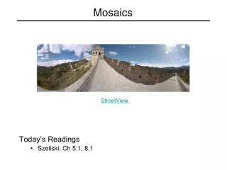
37. Assembling the panorama • Stitch pairs together, blend, then crop

38. Image Compositing Issues • With homography computed, how to render combined image? • Simply putting one image on top of the other, even with bilinear interpolation, may result in a “seam” due to different brightness levels • Auto-iris can change overall lightness of images • Vignetting can make image edges darker courtesy of P. Haeberli

39. Image feathering • Weight each image proportional to its distance from the edge (distance map [Danielsson, CVGIP 1980] • 1. Generate weight map for each image • 2. Sum up all of the weights and divide by sum:weights sum up to 1: wi’ = wi / ( ∑iwi)

40. Image Feathering

41. + = 1 0 1 0 Feathering

42. 0 1 0 1 Effect of window size left right

43. 0 1 0 1 Effect of window size

44. Bilinear Compositing • Idea: Use “hat” function w indicating weight of contributions of an image to the mosaic • w is 1 at source image center, falls linearly to 0 at image boundaries • Combination of horizontal and vertical hat functions: • Normalize hat weights to get blend factor in overlaping area:

45. FUTURE DIRECTIONS

46. Automatic image stitching

47. Local image descriptor • Thresholded image gradients are sampled over 16x16 array of locations in scale space • Create array of orientation histograms (w.r.t. key orientation) • 8 orientations x 4x4 histogram array = 128 dimensions • Normalized, clip values larger than 0.2, renormalize σ=0.5*width

48. Keypoint localization X is selected if it is larger or smaller than all 26 neighbors

50. Feature Matching • Best match is defined as the minimum of the sum of the absolute difference between descriptor vectors.