Download
1 / 20
200 likes | 301 Views
Chapter 10 Dissimilarity Analysis. Presented by: ASMI SHAH (ID : 24). 10.4 Pattern Recognition. Taking an Example of digits display unit in a calculator, the table will be assumed to represent a characterization of “hand written” digits, consist of horizontal and vertical strokes. .

E N D
Chapter 10 Dissimilarity Analysis Presented by: ASMI SHAH (ID : 24)
10.4 Pattern Recognition Taking an Example of digits display unit in a calculator, the table will be assumed to represent a characterization of “hand written” digits, consist of horizontal and vertical strokes.
Table describes each digit in terms of elements a, b, c, d, e, f and g. Our task is to find a minimal description of each digit and the corresponding decision algorithms. Compute the core first and next, find all reducts of attributes. Core is the set {a, b, c, d, e, f, g}
It is sufficient to consider only the attributes {a, b, e, f, g} as the basis for the decision algorithm, which means that there is following dependency between the attribute {a, b, e, f, g} {c, d} Means, c, d are dependent on the reduct so they are not necessary for digits’ recognition. Finding the column reduct
Computing Core for each decision rule, Checking the consistency by removing the attributes. Reduce each decision rule in the table separately, by computing first the core of each rule. Dropping the core value makes the consistent rule inconsistent. • So finding the column reduct first. • Finding the core for each rule. • Computing the Value Reducts for each decision rule.
Removing attribute ‘a’ we get Removing attribute ‘b’ we get Thus removing attribute a makes rule 1, 7 and 4, 9 inconsistent, i.e. we are unable to discern digits 1 and 7, and 4 and 9 without the attribute a. Hence a0 is the core value in rule 1 and 4 whereas a1 is the core value in rules 7 and 9. in which rules (6, 8) and (5, 9) are indiscernible; thus value b0 and b1 are core values in these rules respectively.
Removing attribute ‘e‘ we get Removing attribute ‘f‘ we get we get three pairs of indiscernible rules (2, 3), (5, 6) and (8, 9), which yields core values for corresponding rules (e1, e0), (e0, e1) and (e1, e0). which yields indiscernible pairs (2, 8), and (3, 9) and core values for each pair are (f0, f1).
Finally the last attribute ‘g’removed gives, where pairs of rules (0, 8), and (3, 7) are indiscernible, and the values (g0, g1) and (g1, g0) are cores of corresponding decision rules.
Rules 2, 3, 5, 6, 8 and 9 are already reduced, since these core values discern these rules from the remaining ones, i.e. the rules with the core values only are consistent (true). For the remaining rules, core values make them inconsistent (false), so they do not form reducts and reducts must be computed by adding proper additional attributes to make the rules consistent. Finding Value Reducts for each Row
Reduced Decision Algorithm Because the four decision rules 0, 1, 4 and 7 have two reduced forms, we have altogether 16 minimal decision algorithms. eg’(f’g) 0 a’f’(a’g’) 1 ef’2 e’f’g3 a’f(a’g) 4 b’e’ 5 b’e6 ae’g’(af’g’) 7 befg8 abe’f 9 where x and x’ denote variable and its negation. e1g0 (f1g0) 0 a0f0 (a0g0) 1 e1f0 2 e0f0g1 3 a0f1 (a0g1) 4 b0e0 5 b0e1 6 a1e0 g0 (a1f0g0) 7 b1e1f1g1 8 a1b1e0f1 9 In parenthesis alternative reducts are given.
A better Way for Digits Recognition: a To make the example more realistic assume that instead of seven elements we are given a grid of sensitive pixels, say 9 * 12, in which seven areas marked a, b, c, d, e, f and g as shown in Figure are distinguished. After slight modification the algorithm will recognize much more realistic handwritten digits. b f g c e d
Eg: Buying A Car need minimal description of each car in terms of available features, i.e. we can have to find a minimal decision algorithm as discussed previously.
Where, a – Price b – Mileage c – Size d – Max Speed e – Acceleration and values of attributes are coded as follows: V Price = { low (-), medium (0), high (+) } V Mileage = { low (-), medium (0), high (+) } V Size = { compact (-), medium (0), full (+) } V Max-Speed = { low (-), medium (0), high (+) } V Acceleration = { poor (-), good (0), excellent (+) } The attribute values are coded by symbols in parenthesis.
Compute first the core of attributes. . Removing the attribute a we get Dropping the attribute b we get inconsistent Table which is inconsistent, because of two identical rows 1 and 3 rows 1 and 5 are identical
Removing attributes c, d or e which are consistent.
Thus the core of attributes is the set {a, b}. There are two reducts {a, b, c} and {a, b, e} of the set of attributes, i.e. there are exactly two consistent and independent tables. Thus we have the following dependencies {a,b,c} {d,e} and {a,b,c} {d,c}
Finding the core values for the reduct {a,b,c} It turns out the core values are reducts of the decision rules. So we have the following decision algorithm • a_b0 1 • c_ 2 • a+ 3 • a0c+ 4 • b+ 5 or (price, low) ^ (mileage, medium) 1 (Acceleration, poor) 2 (Price, high) 3 (Acceleration, excellent) 4 (Mileage, high) 5
Thus… Each car is uniquely characterized by a proper decision rule and this characterization can serve as a basis for car evaluation. Knowing differences between various options is often the departure point in deciosion making. The rough set approach seems to be a useful tool to trace the dissimilarities between objects, states, opinions, processes, etc.