Download
1 / 24
240 likes | 245 Views
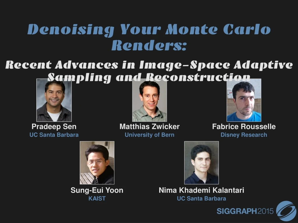
Denoising Your Monte Carlo Renders: Recent Advances in Image-Space Adaptive Sampling and Reconstruction. Pradeep Sen UC Santa Barbara. Matthias Zwicker University of Bern. Fabrice Rousselle Disney Research. Sung- Eui Yoon KAIST. Nima Khademi Kalantari UC Santa Barbara. INTRODUCTION.

E N D
Denoising Your Monte Carlo Renders: Recent Advances in Image-Space Adaptive Sampling and Reconstruction Pradeep Sen UC Santa Barbara Matthias Zwicker University of Bern Fabrice Rousselle Disney Research Sung-Eui Yoon KAIST Nima Khademi Kalantari UC Santa Barbara
INTRODUCTION scene by M. Leal Llaguno
Monte Carlo rendering systems scene by Jesper Lloyd scene by Jesper Lloyd scene by Luca Cugia rendered with LuxRender
Monte Carlo rendering systems • Advantages: • Physically-based results • Flexible and general (all distributed effects) • Little user interaction required • Disadvantages: • Potentially long rendering times • Short rendering times produce noisy images + + + – –
Monte Carlo rendering systems • Distributed Ray Tracing [Cook et al. 1984] • Render MC distributed effects (DoF, area light sources, glossy reflections, etc.) area light diffuse diffuse image real camera glossy ball
Cook et al. [1984] results depth of field motion blur soft shadows glossy reflection
Notable Monte Carlo algorithms • Path tracing [Kajiya 1985] • Bidirectional path tracing [Lafortune & Willems 1994, Veach & Guibas 1994] • Photon mapping [Jensen 1996] • Metropolis light transport [Veach & Guibas 1997]
Monte Carlo integration • Given the definite integral: • We can use this estimator to compute it: • Unbiased estimator: the expected value of this estimator will be equal to the integral
Error in our estimate • Given a number of samples, variance of the estimator will be: • Variance falls off as O(1/N) • Initial samples greatly improve estimate, later they improve it less • Huge problem for rendering…
The problem • Variance appears as noise at low sample rates 16 samples/pixel 4,096 samples/pixel scene by WojciechJarosz
The problem • More objectionable in animated sequences scene by M. Leal Llaguno 8 samples/pixel (1.8 mins/frame)
Previous work to reduce MC noise • There has been over 30 years of research to address this problem • Only provide cursory overview here, please refer to texts on the subject for more info… Pharr and Humphreys [2010] Dutré et al. [2010]
Tracing rays faster • Basic idea: compute samples faster so more samples can be used in estimate • Selected innovations: • Faster intersection algorithms [Kay and Kajiya1986] [Moller and Trumbore 1997] [Havel and Herout2010] • Ray-traversal data structures [Glassner 1984] [Fujimoto et al. 1986] [Arvo and Kirk 1987] [Wald and Harven2006] [Larsson and Akenine-Moller 2003] [Gunther et al. 2007] [Popov et al. 2009] • Memory coherent techniques [Pharr et al. 1997] [Wald et al. 2001, 2006] [Overbecket al. 2008] [Garanzhaand Loop 2010] • Parallel/GPU implementations [Purcell et al. 2002] [Foley and Sugerman2005] [Ailaand Laine2009] [Parker et al. 2010] [van Antwerpen2011] • Dedicated ray tracing hardware [Humphreys and Ananian1996] [Schmittleret al. 2002,2004] [Caustic Graphics 2010] [Nah et al. 2011]
Better sampling techniques • Basic idea: better sampling reduces noise • Selected innovations: • Low discrepancy / Poisson disk [Dippé and Wold 1985] [Cook 1986] [Ulichney 1987] [Shirley 1991] [Kopf et al. 2006] [Wei 2008, 2010] [Lagae and Dutré 2008] [Schmaltz et al. 2012] [Chen et al. 2013] • Quasi Monte Carlo sampling patterns [Shirley 1991] [Keller 1996] [Keller et al. 2002] • Importance sampling [Whitted 1980] [Mitchell 1987, 1996] [Veach and Guibas 1995] [Clarberg et al. 2005], [Ramamoorthi et al. 2007] [Křivánek and Colbert 2008] [Soler et al. 2009]
Efficient MC integration algorithms • Basic idea: reduce variance through better light path sampling • Selected innovations: • Unbiased methods [Kajiya 1986] [Veach and Guibas 1994, 1997] [Lafortune and Willems 1993], [Jakob and Marschner 2012] [Lehtinenet al. 2013] [Hachisuka 2014] • Biased methods [Jensen 1996, 2001] [Keller 1997] [Walter et al. 2005, 2012] [Hachisuka et al. 2008, 2009] [Jarosz et al. 2008] [Knaus and Zwicker 2011] [Hachisuka and Jensen 2011] [Georgiev et al. 2012]
Exploiting properties of integrand • Basic idea: integrand f( ) has properties we can exploit to place or reuse samples • Selected innovations: • Methods exploiting anisotropy [Hachisuka et al. 2008] [Egan et al. 2009, 2011] [Mehta et al. 2012, 2013, 2014] [Lehtinen et al. 2011, 2012] [Munkberg et al. 2014] • Methods exploiting transform domain [Chai et al. 2000] [Ramamoorthi and Hanrahan 2001] [Sloan et al. 2002, 2003], [Durand et al. 2005] [Soler et al. 2009] [Overbeck et al. 2009] [Sen and Darabi 2011] [Belcour et al. 2013]
Better models for specific scenes • Basic idea: efficient algorithms for specific light transport effects and materials • Selected innovations: • Subsurface scattering [Jensen 2001] [Donner and Jensen 2005] [Hašan et al. 2010] [Gkioulekas et al. 2013] • Hair rendering [Marschner et al. 2003] [Selle et al. 2008] [Jakob et al. 2009] [Xu et al. 2011] • Cloth rendering [Zhao et al. 2011, 2012] [Irawan and Marschner 2012] [Sadeghi et al. 2013] • Highly specular scenes [Jakob and Marschner 2012]
So why do we still need this course? • Monte Carlo rendering of complex scenes still takes many hours in production • Algorithmic improvements have been offset by increases in scene complexity • Complicates use of Monte Carlo rendering in production environments • We present approaches orthogonal to many of these previous methods • They work in screen space – independent of scene complexity • Can produce high quality results quickly…
Sample result [Kalantari et al. 2015] Path traced scene Filtered result scene by Jo Ann Elliott 4 samples/pixel (40.8 sec) 4 samples/pixel (48.9 sec) using only post-process filter!
Adaptive sampling + reconstruction • These algorithms use 2 kinds of noise reduction strategies, sometimes combined: • Adaptive sampling algorithms • Use information from renderer to position new samples better to reduce noise • Reconstruction (filtering) algorithms • Use information from renderer to remove MC noise directly • Both methods have been explored in the past!
Previous work on adaptive sampling • Early on, researchers observed potential of adaptively sampling the scene • Large body of work using adaptive sampling to reduce Monte Carlo noise [Mitchell 1987, 1991] [Painter and Sloan 1989] [Bolin and Meyer 1998] [Guo 1998] [Bala et al. 2003] [Hachisuka et al. 2008] [Overbeck et al. 2009] [Soler et al. 2009] [Belcour et al. 2013] • Typically use simple reconstruction kernel (box filter or sheared filter) at the back end • These new methods combine adaptive sampling with complex image-space filters: • Cross-bilateral • Cross non-local means [Mitchell 1987] rendered image sample map
Previous work on filtering • Denoising fully general MC distributed effects [Lee and Redner 1990] [Rushmeier and Ward 1994] • Denoising specific distributed effects: • Illumination noise [Jensen & Christensen 1995] [McCool 1999] [Xu & Pattanaik2005] [Meyer & Anderson 2006] [Segovia et al. 2006] [Laine et al. 2007] [Bauszat et al. 2011] [Egan et al. 2011] • Depth of field or motion blur noise [Egan et al. 2009] [Soler et al. 2009] [Chen et al. 2011] • Real-time illumination [Dammertz et al. 2010] [Mehta et al. 2012, 2013] • Real-time depth of field or motion blur noise [Shirley et al. 2011] [Munkberg et al. 2014] • Real-time illumination + depth of field noise [Mehta et al. 2014] [Bauszat et al. 2015]
New general filtering algorithms • Fully general – work for all distributed effects • Some combine adaptive sampling + filtering [Rousselle et al. 2011, 2012, 2013] [Kalantari and Sen 2013] [Moon et al. 2014] • Others are entirely post-process filters [Sen and Darabi 2011, 2012] [Kalantari and Sen 2015] • Filters using only information from renderer • Work in image space, independent of scene complexity • Biased, but produce high-quality results for offline rendering • Source code for these algorithms is available [Mitchell 1987] rendered image sample map
Course outline • Introduction to general framework for filtering • MC denoising with general image denoising [Kalantari and Sen 2013] • Removing noise from random parameters [Sen and Darabi 2011, 2012] • Cross-bilateral and NL-means filtering with SURE-based error [Rousselle et al. 2012, 2013] • Local weighted regression [Moon et al. 2014] • Learning-based filtering [Kalantari et al. 2015] • Conclusions