Download
1 / 50
500 likes | 563 Views
Plane problems in FEM analysis. from the real system, to the mechanical model, to the mathematical model. from the real system, to the mechanical model, to the mathematical model. F=KD. Introduction. Necessary preliminaries from solid mechanics theory are reviewed.

E N D
from the real system, to the mechanical model, to the mathematical model
from the real system, to the mechanical model, to the mathematical model F=KD
Introduction • Necessary preliminaries from solid mechanics theory are reviewed. • Plane elements of several types are discussed • Particular attention it is posed to element displacement fields and what they portend for element behaviour. • Treatment of loads and calculation of stress are discussed • The application of plane element to the frame structural connection is presented
Two-dimensional Elements • By definition, a plane body is flat and of constant thickness. • Thin or thick plate elements . • Two coordinates to define position. • Elements connected at common nodes and/or along common edges. • Nodal compatibility enforced to obtain equilibrium equations • Two types - Plane stress - Plane strain
y T x Plane stress x,y ,xy 0 z ,xz ,yz = 0 Plate with a Hole y T T x z 0 Plate with a Fillet
A state of stress in which normal stress and shear stresses directed perpendicular to the plane of the body are assumed to be zero. • If x-y plane is plane of body then only nonzero stresses are: x,y ,xy • Zero stresses: z ,xz ,yz • Stresses act in the plane of the plate and can be called membrane stresses. They are constant through the z-direction • The deformation field is tridimensional (ez0 ), the thickness is free to increase or decrease in response to stress in xy plane. • The component of the deformation perpendicular to the plane of the body is due to the transversal contraction (Poisson effect). As the thickness of a plane body increase, from much less to greater than in-plane conditions of the body, there is a transition of behaviour from plane stress toward plane strain
y x z Dam Subjected to Horizontal Load Plane strain y x , y , xy 0 z , xz , yz = 0 x Pipe subjected to externalpressure on its surface z z 0
A state of strain in which normal strain and shear strains directed perpendicular to the plane of the body are assumed to be zero. • If x-y plane is plane of body then only nonzero strains are: x , y , xy • Zero strains: z , xz , yz • Two principal stresses act in plane of the body • The third principal stress, perpendicular to the plane of the body, depends on the first two principal stresses and on the Poisson coefficient • The value of the third principal stress guarantee the deformation perpendicular to plane of the body is zero and prevent thickness change. • Stresses are constant through the z-direction
Two-dimensional State of Stress y xy y xy xy dy x x x dx xy y
Principal stresses 2 1 P 1 x 2
Two-dimensional State of Strain y, v D B A x, u Displacements and rotations of lines of an element in the x-y plane
Constitutive relation Let the material linearly elastic and isotropic E = elastic modulus = Poisson coefficient
Plane stress x,y ,xy 0 z ,xz ,yz = 0
x , y , xy 0 z , xz , yz = 0 Plane strain
Strain-displacement relations FE theory makes extensive use of strain-displacement relations to obtain the strain field from a displacement field The strain definitions suitable if the material has small strains and small rotations are
Displacement interpolation Displacements in a plane FE are interpolated from nodal displacement u(x,y), and v(x,y) as follow: where N is the shape function matrix
According to the previous equation • u depends only on the ui • v depends only on the vi • u and v use the same interpolation polynomials • This is a common arrangement but it is not mandatory • From the strain definition, we obtain where B is the strain-displacement matrix
The general formula for k The strain energy per unit volume of an elastic material in terms of strain and in matrix format is: Upon integrating over element volume V and substituting from we obtain: where the element stiffness matrix is For a given E, the nature of k depends entirely on B , the behavior of an element is governed by its shape functions.
Let any element d.o.f. , say the i-th d.o.f., be increased from zero to the value di. • This is accomplished by applying to the d.o.f. a force that increases from zero to Fi.. • The work is Fidi/2, just as it would be stretching a linear spring as amount di. • This work is stored as strain energy U. • The previous equation says that work Fidi/2 is equal to strain energy in the element when the displacement field is that produced by di and the element shape functions. • Example: if di = u1, we can see that the element displacement field is u(x,y)=N1u1 and v(x,y) =0.
Nature of the FE approximation • Stresses are in general functions of the coordinates, so that each stress has a rate of change with respect to x and y. • In a plane problem the rate of change satisfy the equilibrium equations • where Fx and Fy are body forces per unit volume. • As for deformation, they are called compatible if displacement boundary conditions are met and material does not crack apart or overlap itself. • If displacement and stress fields satisfy equilibrium, compatibility, and boundary conditions on stress, then the solution is exact.
How is the exact solution approached by FEA? • Let be elements based on polynomial displacement fields, as for most elements in common use: • - the compatibility requirement is satisfied exactly within elements • - equilibrium equations and boundary conditions on stress are satisfied in average sense • - at most point within the FEA model the equilibrium equations are not satisfied • - as a mesh is repeatedly refined, pointwise satisfaction is approached more and more closely • NOTE This discussion also applies to three-dimensional elastic problems.
Triangular Elements • Two degrees-of-freedom per node. • These are x and y displacements. • ui - x displacement at ith node. • vi - y displacement at ith node. y y m T T j i x x Discretized Plate Using Triangular Elements Thin Plate in Tension
Constant strain triangle (CST) The CST element is the earliest and simplest finite element 3 nodes numbered counterclockwise! 6 d.o.f. 3 (x3, y3) y 1 (x1, y1) 2 (x2, y2) x
Funzioni di spostamento lineare In terms of generalized coordinates bi, (equal to the d.o.f. of the element) its displacement field is • Ensures compatibility between elements. • Displacements vary linearly along any line. • Displacements vary linearly between nodes. • Edge displacements are the same for adjacent elements if nodal displacements are equal.
Strain field The resulting strain field is: • We see that strain do not vary within the element; hence the name “constant strain triangle”. • The element also be called “linear triangle”, because its displacement field is linear in x and y. • Element sides remain straight as the element deform.
The strain field obtained from the shape function, in the form is: Were xi and yi are nodal coordinates (i=1,2,3) xij = xi-xj yij = yi-yj 2A= x21y31-x31y21 is twice the area of the triangle The sequence 123 must go counterclockwise around the element if the area of the element (A) is to be positive.
Stiffness matrix The stiffness matrix for the element is: Were t is the element thickness (plain stress conditions) The integration to obtain K is trivial because B and E contain only constants
Observations The CST gives good results in a region of the FE model where there is little strain gradient. Otherwise it does not work well. Stress along the x axis in a beam modeled by CSTs and loaded in pure bending • This is evident if we ask the CSTR element to model pure bending: • The x-axis should be stress-free because it is the neutral axis; • The FE model predicts sx as a square wave pattern. • The element results enable to represent an ex that varies linearly with y
CST also develop a spurious shear stress when bent: - v2 creates a shear stress that should not be present Despite defects of CST, correct results are approached as a mesh of CST elements is repeatedly refined
v3 u3 3 v4 v5 u4 4 v2 u5 5 v1 u2 v6 2 u6 6 u1 1 Linear stress triangle 6 nodes 12 d.of. The LST element has midside nodes in addition to vertex nodes. The d.o.f. are ui and vi at each node i, i=1,2,…6, for a total of 12 d.o.f.
In terms of generalized coordinates biits displacement field is and the resulting strain field is The strain field can vary linearly with x and y within the element, hence the name “linear strain triangle” (LST). The element may also be called a “quadratic triangle” because its displacement field is quadratic in x and y
Shape function Displacement modes associated with nodal d.o.f. v2=1 and v5=1 • LST has all the capability of CST, few they are, and more. • The strain ex can vary linearly with y • If problem of pure bending is solved, exact results for deflection and stresses are obtained
Comparison of CST and LST Elements 4 Constant Strain Triangles 6 Nodes 12 D-O-F 1 Linear Strain Triangle 6 Nodes 12 D-O-F
4 x 16 mesh 480 mm 120 mm Parabolic Load 40 kN (Total)
Bilinear Quadrilater (Q4) The Q4 element has 4 nodes and 8 d.o.f. 8 d.o.f. In terms of generalized coordinates biits displacement field is
Strain field • The name bilinear arise because the form of the expression for u and v is the product of two linear polynomials • where ci are constants The element strain field is
Cannot exactly model a state of pure bending, despite its ability to represent an ex that varies linearly with y. • Correct deformation mode of a rectangular block in pure bending: • Plain section remain plane • Top and bottom edges became arcs of practically the same radius • Shear strain gxy is absent • Deformation of a bilinear quadrilater under bending load: • Top and bottom edges remain straight • Right angles are not preserved under pure moment load • Shear strain appear everywhere (y0) Q4 element that bent also develop shear strain
Cannot model a cantilever beam under transverse shear force where the moment and the axial strain ex vary linearly with x. Qualitative variation of axial stress and average transverse shear stress Q4 element results too stiff in bending because an applied bending moment is resisted by spurious shear stress as well as by the expected flexural stresses (locking)
Shape functions If the generalized coordinates bi are expressed in terms of nodal d.o.f.,we obtain the displacement field in the form where Shape function N2
Strain field The element strain field is • Equilibrium is not satisfied at every point unless b4 = b8 = 0 (constant strain) • The element converges properly with mesh refinement and in most problem it works better than the CST element which always satisfied the equilibrium equations • Non rectangular shape are permitted.
Comparative examples a a • The test problem chosen here is that of a cantilever beam of unit thickness loaded by a transverse tip force. • Plane stress conditions prevail. • Support conditions are consistent with a fixed end but without restraint of y-direction deformation associated with the Poisson effect.
Results • Simple beam element solves the problem exactly when transverse shear deformation is included in the formulation. • As expected, CST elements perform poorly. • Q4 element are better but not good. • LST elements give an accurate deflection but a disappointing stress. Distortion and elongation of elements are seen to reduce accuracy
Elementi quadrilateri a 8 nodi (Q48) The Q8 element has midside nodes in addition to vertex nodes. The d.o.f. are ui and vi at each node i, i=1,2,…8, for a total of 16 d.o.f. 16 g.d.l. In terms of generalized coordinates biits displacement field is
Shape functions (Q8) The displacement field in terms of shape function is As examples, two of the eight shape functions are The displacements are quadratic in y, which means that the edge deform into a parabola when a single d.o.f on that edge is nonzero.
Strain field The element strain field is : (no term in x2) …. • Q8 element can represent exactly all states of constant strain, and state of pure bending, if it is rectangular. • Non rectangular shape are permitted.
Final comparison a Q8 elements are the best performers a