Download
1 / 64
650 likes | 1.09k Views
Safety Inventories. Chapter 11 of Chopra. Why to hold Safety Inventory?. Desire for quick product availability Ease of search for another supplier “ I want it now ” culture Demand uncertainty Short product life cycles Safety inventory. Measures . Measures of demand uncertainty

E N D
Safety Inventories Chapter 11 of Chopra
Why to hold Safety Inventory? • Desire for quick product availability • Ease of search for another supplier • “I want it now” culture • Demand uncertainty • Short product life cycles • Safety inventory
Measures • Measures of demand uncertainty • Variance of demand • Ranges for demand • Delivery Lead Time, L • Measures of product availability • Stockout, what happens? • Backorder (patient customer, unique product or big cost advantage) or Lost sales. • I. Cycle service level(CSL), % of cycles with no stockout • II. Product fill rate (fr), % of products sold from the shelf • Order fill rate, % of orders • Equivalent to product fill rate if orders contain one product
Service measures: CSL and fr are different inventory CSL is 0%, fill rate is almost 100% 0 time inventory CSL is 0%, fill rate is almost 0% 0 time
Replenishment policies • When to reorder? • How much to reorder? • Most often these decisions are related. Continuous Review: Order fixed quantity when total inventory drops below Reorder Point (ROP). - ROP meets the demand during the lead time L. - One has to figure out the ROP. Information technology facilitates continuous review.
Normal Density Function frequency normdist(x,.,.,1) normdist(x,.,.,0) Prob x Mean 95.44% 99.74%
Cumulative Normal Density 1 prob normdist(x,mean,st_dev,1) 0 x norminv(prob,mean,st_dev)
Demand During Lead Time Determines ROP Suppose that demands are identically and independently distributed. To mean identically and independently distributed, use iid. F is the cumulative density function of the demand in a single period, say a day. The second equality above holds if demand is Normal.
Optimal Safety Inventory Levels inventory An inventory cycle Q ROP time Lead Times Shortage
I. Cycle Service Level: ROP CSL Cycle service level: percentage of cycles with stock out ROP: Reorder point
I. Cycle Service Level for Normal Demands The last equality is a property of the Normal distribution.
Example: Finding CSL for given ROP R = 2,500 /week; = 500 L = 4 weeks; Q = 10,000; ROP = 16,000 ss = ROP – L R = Cycle service level, Average Inventory = Average Flow Time =Average inventory/Thruput= If you wish to compute Average Inventory = Q/2 + ss
Safety Inventory: CSL ROP The last two equalities are by properties of the Normal distribution. Very important remark: Safety inventory is a more general concept. It exists without lead time. It is the stock held minus the expected demand.
Finding ROP for given CSL R = 2,500/week; = 500 L = 4 weeks; Q = 10,000; CSL = 0.90 Factors driving safety inventory • Replenishment lead time • Demand uncertainty
II. Fill rate:Expected shortage per cycle • ESCis the expected shortage per cycle • ESC is not a percentage, it is the number of units, also see next page
Inventory and Demand during Lead Time ROP 0 Inventory= ROP-DLT ROP Upside down Inventory 0 DLT: Demand During LT LT 0 Demand During LT
Shortage and Demand during Lead Time ROP 0 Shortage= DLT-ROP ROP Upside down DLT: Demand During LT 0 Shortage LT 0 Demand During LT
Expected shortage per cycle • First let us study shortage during the lead time • Ex:
Expected shortage per cycle • Ex: If demand is normal: • Does ESC decrease or increase with ss, L? • Does ESC decrease or increase with expected value of demand?
Fill Rate • Fill rate: Proportion of customer demand satisfied from stock • Q: Order quantity
Finding the Fill Ratess fr = 500; L = 2 weeks; ss=1000; Q = 10,000; Fill Rate (fr) = ? fr = (Q - ESC)/Q = (10,000 - 25.13)/10,000 = 0.9975.
Finding Safety Inventory for a Fill Rate: fr ss If desired fill rate is fr = 0.975, how much safety inventory should be held? Clearly ESC = (1 - fr)Q = 250 Try some values of ss or use goal seek of Excel to solve
Evaluating Safety Inventory For Given Fill Rate Safety inventory is very sensitive to fill rate. Is fr=100% possible?
Factors Affecting Fill Rate • Safety inventory: If Safety inventory is up, • Fill Rate is up • Cycle Service Level is up. • Lot size: If Lot size Q is up, • Cycle Service Level does not change. Reorder point, demand during lead time specify Cycle Service Level. • Expected shortage per cycle does not change. Safety stock and the variability of the demand during the lead time specify the Expected Shortage per Cycle. Fill rate is up.
To Cut Down the Safety Inventory • Reduce the Supplier Lead Time • Faster transportation • Air shipped semiconductors from Taiwan • Better coordination, information exchange, advance retailer demand information to prepare the supplier • Textiles; Obermeyer case • Space out orders equally as much as possible • Reduce uncertainty of the demand • Contracts • Better forecasting to reduce demand variability
Lead Time Variability Supplier’s lead time may be uncertain: The formulae do not change:
Impact of Lead Time Variability, s R = 2,500/day; = 500 L = 7 days; Q = 10,000; CSL = 0.90
Methods of Accurate Response to Variability • Centralization • Physical, Laura Ashley • Information • Virtual aggregation, Barnes&Nobles stores • Specialization, what to aggregate • Product substitution • Raw material commonality - postponement
Centralization: Inventory Pooling Which of two systems provides a higher level of service for a given safety stock? Consider locations and demands: With k locations centralized, mean and variance of
Sum of Random Variables Are Less Variable When they are independent, cov(Di,Dj)=0 When they are perfectly positively correlated, cov(Di,Dj)=σi σj When they are perfectly negatively correlated, cov(Di,Dj)= - σiσj
Factors Affecting Value of Aggregation • When to aggregate? Statistical checks: Positive correlation and Coefficient of Variation. • Aggregation reduces variance almost always except when products are positively correlated • Aggregation is not effective when there is little variance to begin with. When coefficient of variation of demand is relatively small (variance w.r.t. the mean is small), do not bother to aggregate. • In real life, • Is the electricity demand in Arlington and Plano are positively or negatively correlated? Is there an underlying factor which affects both in the same direction? Note that a big portion of electricity is consumed for heating/cooling. • Are the Campbell soup sales over time positively or negatively correlated? How many soups can you drink per day?
Impact of Correlation on Aggregated Safety Inventory (Aggregating 4 outlets) • Safety stocks are proportional to the StDev of the demand. • With four locations, we have total ss proportional to 4*σ • If four locations are all aggregated, • ss proportional to 4*σ with correlation 1 • ss proportional to 2*σ with correlation 0 • Benefit=SS before - SS after / SS before
Impact of Correlation on Aggregated Safety Inventory (Aggregating 4 outlets) • Benefit=(SS before - SS after) / SS before
EX 11.8: W.W. Grainger a supplier of Maintenance and Repair products • About 1600 stores in the US • Produces large electric motors and industrial cleaners • Each motor costs $500; Demand is iid Normal(20,40x40) at each store • Each cleaner costs $30; Demand is iid Normal(1000,100x100) at each store • Which demand has a larger coefficient of variation? • How much savings if motors/cleaners inventoried centrally?
Use CSL=0.95 Supply lead time L=4 weeks for motors and cleaners For a single store Motor safety inventory=Norminv(0.95,0,1) 2 (40)=132 Cleaner safety inventory=Norminv(0.95,0,1) 2 (100)=329 Value of motor ss=1600(132)(500)=$105,600,000 Value of cleaner ss=1600(329)(30)=$15,792,000 Standard deviation of demands after aggregating 1600 stores Standard deviation of Motor demand=40(40)=1,600 Standard deviation of Cleaner demand=40(100)=4,000 For the aggregated store Motor safety inventory=Norminv(0.95,0,1) 2 (1600)=5,264 Cleaner safety inventory=Norminv(0.95,0,1) 2 (4,000)=13,159 Value of motor ss=5264(500)=$2,632,000 Value of cleaner ss=13,159(30)=$394,770
EX. 11.8: Specialization: Impact of cv on Benefit From 1600-Store Aggregation , h=0.25
Slow vs Fast Moving Items • Low demand = Slow moving items, vice versa. • Repair parts are typically slow moving items • Slow moving items have high coefficient of variation, vice versa. • Stock slow moving items at a central store Buying a best seller at Amazon.com vs. a Supply Chain book vs. a Banach spaces book, which has a shorter delivery time? - Why cannot I find a “driver-side-door lock cylinder” for my 1994 Toyota Corolla at Pep Boys? - Your instructor on March 26 2005. • “Case Interview books” are not in our s.k.u. list. You must check with our central stores. • Store keeper at Barnes and Nobles at Collin Creek, March 2002.
Product Substitution • Manufacturer driven • Customer driven Consider: The price of the products substituted for each other and the demand correlations • One-way substitution • Army boots. What if your boot is large? Aggregate? • Two-way substitution: • Grainger motors; water pumps model DN vs IT. • Similar products, can customer detect specifications. If products are very similar, why not to eliminate one of them?
Component Commonality. Ex. 11.9 • Dell producing 27 products with 3 components (processor, memory, hard drive) • No product commonality: A component is used in only 1 product. 27 component versions are required for each component. A total of 3*27 = 81 distinct components are required. • Component commonality allows for component inventory aggregation.
Max Component Commonality • Only three distinct versions for each component. • Processors: P1, P2, P3. Memories: M1, M2, M3. Hard drives: H1, H2, H3 • Each combination of components is a distinct product. A component is used in 9products. • Each way you can go from left to right is a product. H1 P1 M1 Left Right H2 P2 M2 H3 M3 P3
Example 11.9: Value of Component Commonalityin Safety Inventory Reduction # of products a component is used in Aggregation provides reduction in total standard deviation.
Standardization • Standardization • Extent to which there is an absence of variety in a product, service or process • The degree of Standardization? • Standardized products are immediately available to customers • Who wants standardization? • The day we sell standard products is the day we lose a significant portion of our profit • A TI manager on November 1, 2005
Advantages of Standardization • Fewer parts to deal with in inventory & manufacturing • Less costly to fill orders from inventory • Reduced training costs and time • More routine purchasing, handling, and inspection procedures • Opportunities for long production runs, automation • Need for fewer parts justifies increased expenditures on perfecting designs and improving quality control procedures.
Disadvantages of Standardization • Decreased variety results in less consumer appeal. • Designs may be frozen with too many imperfections remaining. • High cost of design changes increases resistance to improvements • Who likes optimal Keyboards? • Standard systems are more vulnerable to failure • Epidemics: People with non-standard immune system stop the plagues. • Computer security: Computers with non-standard software stop the dissemination of viruses. • Another reason to stop using Microsoft products!
Inventory–Transportation Costs: Eastern Electric Corporation: p.427 • Major appliance manufacturer, buys motors from Westview motors in Dallas • Annual demand = 120,000 motors • Cost per motor = $120; Weight per motor 10 lbs. • Current order size = 3,000 motors • 30,000 pounds = 300 cwt • 1 cwt = centum weight = 100 pounds; Centum = 100 in Latin. • Lead time = 1 + the number of days in transit • Safety stock carried = 50% of demand during delivery lead time • Holding cost = 25% • Evaluate the mode of transportation for all unit discounting based on shipment weight
AM Rail proposal: Over 20,000 lbs at 0.065 per lb in 5 days • For the appliance manufacturer • No fixed cost of ordering besides the transportation cost • No reason to transport at larger lots than 2000 motors, which make 20,000 lbs. • Cycle inventory=Q/2=1,000 • Safety inventory=(6/2)(120,000/365)=986 • In-transit inventory • All motors shipped 5 days ago are still in-transit • 5-days demand=(120,000/365)5=1,644 • Total inventory held over an average day=3,630 motors • Annual holding cost=3,630*120*0.25=$108,900 • Annual transportation cost=120,000(10)(0.065)=$78,000
Inventory–Transportation trade off: Eastern Electric Corporation, see p.426-8 for details If fast transportation not justified cost-wise, need to consider rapid response
Physical Inventory Aggregation: Inventory vs. Transportation cost: p.428 • HighMed Inc. producer of medical equipment sold directly to doctors • Located in Wisconsin serves 24 regions in USA • As a result of physical aggregation • Inventory costs decrease • Inbound transportation cost decreases • Inbound lots are larger • Outbound transportation cost increases
Inventory Aggregation at HighMed Highval ($200, .1 lbs/unit) demand in each of 24 territories • H = 2, H = 5 Lowval ($30/unit, 0.04 lbs/unit) demand in each territory • L = 20, L = 5 UPS rate: $0.66 + 0.26x {for replenishments} FedEx rate: $5.53 + 0.53x {for customer shipping} Customers order 1 H + 10 L