Failure Patterns

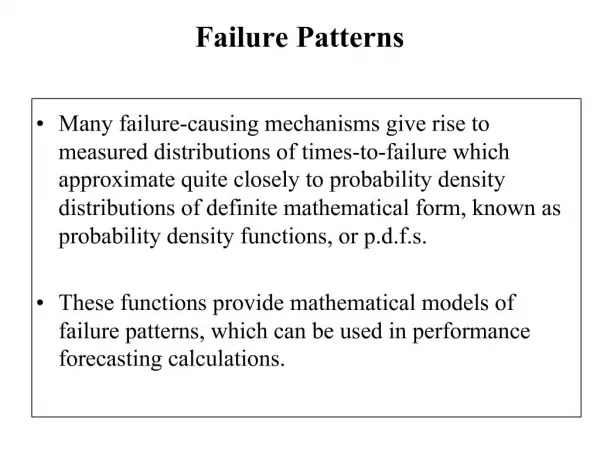
1. Failure Patterns • Many failure-causing mechanisms give rise to measured distributions of times-to-failure which approximate quite closely to probability density distributions of definite mathematical form, known as probability density functions, or p.d.f.s. • These functions provide mathematical models of failure patterns, which can be used in performance forecasting calculations.

2. Some Known Failure Patterns • The negative exponential p.d.f • The hyper-exponential or " running-in' p.d.f • The normal or 'wear-out' p.d.f

3. Negative Exponential p.d.f • A very wide range of components and equipment shows that, under normal operating conditions and during their normal operating life do not reach a point of wear-out failure at some likely time that could be called "old age". • However, they are likely to fail in a given week shortly after installation as in a given week many months later. • The probability of failure is constant and independent of running time; the item is always effectively 'as good as new'.

4. Negative Exponential p.d.f In this case the p.d.f is: ƒ(t) = λ exp (- λt) where: λ = average failure rate (failures/ unit time) per machine. 1/λ = average time to failure

5. Hyper-Exponential or " Running-in' p.d.f • Many equipment the probability of failure is fund to be much higher during the period following installation (results from built-in defects that show up during the running –in stage) than during its subsequent useful life.

6. Hyper-Exponential or " Running-in' p.d.f The p.d.f of time-to –failure in this case, exhibits two phases: • an initial rapid exponential fall. • with a later slower exponential fall.

7. Normal or ‘Wear-out' p.d.f • Equipment that show a marked wear-out failure pattern, tend to fail at some mean operating age, m, with some failing sooner and some later, thus giving dispersion, of standard deviation s, in the recorded times to failure.

8. Negative Exponential p.d.f In this case the p.d.f of time- to –failure is: ƒ(t) = 1/ s√(2π) exp {- ((t-m)²/ 2s²)} • This is a normal p.d.f where 50% of all items would expected to show time to failure in range (m-0.67s) to (m+0.67s), 95% in the range (m-2s) to (m+2s).

9. Normal or ‘Wear-out' p.d.f • The different areas under the normal distribution curve represent probabilities of certain cases. • They are fund by calculating the number x of standard deviations above the mean value, m. • This means that to find the probability associated with a given time t, to failure the associated value of x should be calculated by using: x = t- m / s

10. Failure Probability, Survival Probability, Age-Specific Failure Rate • Failure probability: is the fraction of items which can be expected to fail by the running time, t , since new. F(t) = probability of failure before a running time t. F(t) = ∫ ƒ(t)dt • For the negative exponential p.d.f : F(t) = ∫ λ exp(-λt)dt = 1 – exp(-λt)

11. Failure Probability, Survival Probability, Age-Specific Failure Rate • Survival probability: is the fraction of items surviving at running time t. P(t) = survival probability, at time t, for any one item or it is called the reliability of the item at time t. P(t) = 1 – F(t) • For the negative exponential p.d.f : P(t) = exp(-λt)

12. Failure Probability, Survival Probability, Age-Specific Failure Rate • Age-specific failure rate: is the fraction, Z(t), of those items which have survived up to the time, t, which can be expected to fail in the next unit of time. • Some it is called instantaneous failure rate, local failure rate, local probability of failure, hazard function, or failure rate. Z(t) = ƒ(t)/ P(t) =ƒ(t)/ 1-F(t) • For the negative exponential : Z(t) = λ exp (-λt)/ exp (-λt) = λ

13. Weibull p.d.f • a single p.d.f which can be made to represent any of the three types of p.d.f.s of times-to-failure (running-in, purely random, or wear-out modes of failure). • meaningful parameters of failure pattern, such as probable minimum time to failure. • simple graphical techniques for its practical application.

14. Weibull p.d.f • The form of the c.d.f is : F(t) = 1- exp (-ø(t)) • Where: ø(t) = function of time to failure which has a definite form. This form should be: • F(t) should never decrease as t increase. • F(t) should be zero at some threshold time to. • ø(t) should be dimensionless (since it is an exponent).

15. Weibull p.d.f • The suggested form of ø(t) that satisfies these conditions is: ø(t) = { t- t۪ / ŋ} and the c.d.f for the time-to-failure is: F(t) = 1 – exp { - (t- t۪ / ŋ)

16. Weibull p.d.f • The survival or the reliability function, the p.d.f and the failure rate are: P(t) = exp { - (t- t۪ / ŋ) } ƒ(t) = (β(t – t۪) / ŋ ) exp { - (t- t۪ / ŋ) } Z(t) = (β/ ŋ ) (t – t۪) (non-zero and rising only after t۪)

17. Weibull p.d.f Where: T۪ = the threshold time-to-failure, or guaranteed life. In many cases of wear-out the first failure do not appear until some significant running time t۪ has elapsed. ŋ = the characteristic life. When t – t۪ = ŋ , P(t) = exp (-1) = 0.37, ŋ is the interval between t۪ and the time at which it can be expected that 63% of the items will have failed. β = the shape factor. In the case of a "running-in" or "infant –morality" failure pattern, it is less than one and in the case of a wear-out failure patterns, it is has larger values (say larger than 3). whereas, in the case of "random failure' pattern and, it is fairly close to one. Also if β less than 3, a purely random failure pattern is still significant.

18. Application of Failure Statistics to Maintenance and Reliability Engineering • One of its application is in the provision to designers and reliability engineers, enabling them to determine system reliabilities, availabilities and expected lives. • It is also useful to maintenance engineers and managers in two main ways: a. in the diagnosis of the nature of a recurrent equipment failure. b. in the prescription of solutions to maintenance problems.