PCA and eigenfaces

1. PCA and eigenfaces T-11 Computer Vision University of Ioannina Christophoros Nikou Images and slides from: James Hayes, Brown University, Computer Vision course D. Forsyth and J. Ponce. Computer Vision: A Modern Approach, Prentice Hall, 2003. Computer Vision course by Svetlana Lazebnik, University of North Carolina at Chapel Hill. Computer Vision course by Michael Black, Brown University. Research page of Antonio Torralba, MIT.

2. Face detection and recognition

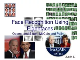
3. Face detection and recognition Detection Recognition “Sally”

4. Consumer application: iPhoto 2009 http://www.apple.com/ilife/iphoto/

5. Consumer application: iPhoto 2009 It can be trained to recognize pets! http://www.maclife.com/article/news/iphotos_faces_recognizes_cats

6. Consumer application: iPhoto 2009 iPhoto decides that this is a face

7. Outline • Face recognition • Eigenfaces • Face detection • The Viola and Jones algorithm. M. Turk and A. Pentland. "Eigenfaces for recognition". Journal of Cognitive Neuroscience, 3(1):71–86, 1991. Also in CVPR 1991. P. Viola and M. Jones. Robust real-time face detection. International Journal of Computer Vision, 57(2), 2004. Also in CVPR 2001.

9. The space of all face images • When viewed as vectors of pixel values, face images are extremely high-dimensional • 100x100 image = 10,000 dimensions • However, relatively few 10,000-dimensional vectors correspond to valid face images. • Is there a compact and effective representation of the subspace of face images?

10. The space of all face images • Insight into principal component analysis (PCA). • We want to construct a low-dimensional linear subspace that best explains the variation in the set of face images.

11. Principal Component Analysis • Given: N data points x1, … ,xNin Rd • We want to find a new set of features that are linear combinations of the original ones:w(xi) = uT(xi – µ)(µ: mean of data points) • What unit vector uin Rd captures the most variance of the data?

12. Principal Component Analysis • The variance of the projected data: Projection of data point Covariance matrix of data

13. We nowestimate vector u maximizing the variance: Principal Component Analysis subject to: because any multiple of u maximizes the objective function. • The Lagrangian is leading to the solution: which is the eigenvector corresponding to the largest eigenvalue of Σ.

14. Principal Component Analysis • The direction that captures the maximum covariance of the data is the eigenvector corresponding to the largest eigenvalue of the data covariance matrix. • The top k orthogonal directions that capture the most variance of the data are the k eigenvectors corresponding to the k largest eigenvalues.

15. Principal Component Analysis • By using all of the d eigenvectors, we transform the original data into a new orthogonal basis: • Most important: we may recover the original coordinates as a linear combination of the eigenvectors:

16. Principal Component Analysis The above is true because the eigenvectors of a symmetric positive semi-definite matrix are orthonormal: and

17. Principal Component Analysis • Property: the covariance matrix of the transformed data is diagonal • The transformed data are decorrelated:

18. Eigenfaces: Key idea • Assume that most face images lie on a low-dimensional subspace determined by the first k (k<d) directions of maximum variance. • Use PCA to determine the vectors or “eigenfaces” u1,…ukthat span that subspace. • Represent all face images in the dataset as linear combinations of eigenfaces.

19. Eigenfaces example Training images

20. Eigenfaces example Top eigenvectors Mean: μ

21. Eigenfaces example • Face x in “face space” coordinates: • Reconstruction: = +

22. Eigenfaces example • Any face of the training set may be expressed as a linear combination of a number of eigenfaces. • In matrix-vector form: Approximation error: = +

23. Eigenfaces example

24. Eigenfaces example Intra-personal subspace (variations in expression) Extra-personal subspace (variations between people)

25. Face Recognition with eigenfaces Process the training images: • Find mean µ and covariance matrix Σ. • Find k principal components (eigenvectors of Σ) u1,…uk. • Project each training image xi onto subspace spanned by principal components:(wi1,…,wik) = (u1T(xi – µ), … , ukT(xi– µ)) Given a new image x: • Project onto subspace:(w1,…,wk) = (u1T(x– µ), … , ukT(x– µ)). • Optional: check the reconstruction error x – x to determine whether the new image is really a face. • Classify as closest training face in k-dimensional subspace. ^ M. Turk and A. Pentland, Face Recognition using Eigenfaces, CVPR 1991

26. Application: MRF features for texture representation

27. Application: view-based modeling • PCA on various views of a 3D object. H. Murase and S. Nayar. Visual Learning and Recognition of 3D objects from appearance, International Journal of Computer Vision, Vol. 14, pp. 5-24,1995.

28. Application: view-based modeling • Subspace of the first three PC (varying view angle). H. Murase and S. Nayar. Visual Learning and Recognition of 3D objects from appearance, International Journal of Computer Vision, Vol. 14, pp. 5-24,1995.

29. Application: view-based modeling • View angle recognition. H. Murase and S. Nayar. Visual Learning and Recognition of 3D objects from appearance, International Journal of Computer Vision, Vol. 14, pp. 5-24,1995.

30. Application: view-based modeling • Extension to more 3D objects with varying pose and illumination. H. Murase and S. Nayar. Visual Learning and Recognition of 3D objects from appearance, International Journal of Computer Vision, Vol. 14, pp. 5-24,1995.

31. Limitations • Global appearance method • not robust to misalignment, background variation.

32. Limitations • Projection may suppress important detail • The smallest variance directions may not be unimportant. PCA assumes Gaussian data. The shape of this dataset is not well described by its principal components

33. Limitations • PCA does not take the discriminative task into account • Typically, we wish to compute features that allow good discrimination. • Projection onto the major axis can not separate the green from the red data. • The second principal component captures what is required for classification.

34. Canonical Variates • Also called “Linear Discriminant Analysis” • A labeled training set is necessary. • We wish to choose linear functions of the features that allow good discrimination. • Assume class-conditional covariances are the same. • We seek for linear feature maximizing the spread of class means for a fixed within-class variance.

35. Canonical Variates • We have a set of vectorized images xi (i=1,2…,N). • The images belong toC categories each having a mean μj, ( j=1,2,…,C ). • The mean of the class means:

36. Canonical Variates • Between class covariance: with Ni being the number of images in class i. • Within class covariance:

37. Canonical Variates Using the same argument as in PCA (and graph-based segmentation) we seek vector u maximizing which is equivalent to s.t. The solution is the top eigenvector of the generalized eigenvalue problem:

38. Canonical Variates • 71 views of 10 objects at a variety of poses at a black background. • 60 images were used to determine a set of canonical variates. • 11 images were used for testing.

39. Canonical Variates • The first two canonical variates. The clusters are tight and well separated (a different symbol per object is used). • We could probably get a quite good classification.