Download
1 / 7
90 likes | 481 Views
Feynman and his diagrams. Feynman diagrams are pictorial representations of AMPLTUDES of particle reactions, i.e scatterings or decays. Use of Feynman diagrams can greatly reduce the amount of computation involved in calculating a rate or cross section of a physical process, e.g.

E N D
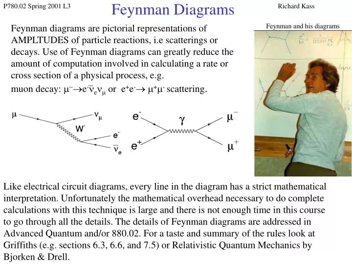
Richard Kass Feynman and his diagrams Feynman diagrams are pictorial representations of AMPLTUDES of particle reactions, i.e scatterings or decays. Use of Feynman diagrams can greatly reduce the amount of computation involved in calculating a rate or cross section of a physical process, e.g. muon decay: m-®e-nenm or e+e-®m+m- scattering. Feynman Diagrams Like electrical circuit diagrams, every line in the diagram has a strict mathematical interpretation. Unfortunately the mathematical overhead necessary to do complete calculations with this technique is large and there is not enough time in this course to go through all the details. The details of Feynman diagrams are addressed in Advanced Quantum and/or 880.02. For a taste and summary of the rules look at Griffiths (e.g. sections 6.3, 6.6, and 7.5) or Relativistic Quantum Mechanics by Bjorken & Drell.
Richard Kass Each Feynman diagram represents an AMPLITUDE (M). Quantities such as cross sections and decay rates (lifetimes) are proportional to |M|2. The transition rate for a process can be calculated using time dependent perturbation theory using Fermi’s Golden Rule: Feynman Diagrams In lowest order perturbation theory M is the fourier transform of the potential. This is the Born approximation. The differential cross section for two body scattering (e.g. pp®pp) in the CM frame is: qf=final state momentum vf= speed of final state particle vi= speed of initial state particle M&S B.29, p296 The decay rate (G) for a two body decay (e.g. K0®p+p-) in CM is given by: m=mass of parent p=momentum of decay particle S=statistical factor (fermions/bosons) Griffiths 6.32 In most cases |M|2 cannot be calculated exactly. Often M is expanded in a power series. Feynman diagrams represent terms in the series expansion of M.
Richard Kass Feynman diagrams plot time vs space: Moller Scattering e-e-®e-e- Feynman Diagrams e- e- M&S style QED Rules Solid lines are charged fermions electrons or positrons (spinor wavefunctions) Wavy (or dashed) lines are photons Arrow on solid line signifies e- or e+ e- arrow in same direction as time e+ arrow opposite direction as time At each vertex there is a coupling constant Öa, a= 1/137=fine structure constant All quantum numbers are conserved at vertex e.g. electric charge, lepton number “Virtual” Particles do not conserve E, p virtual particles are internal to diagram(s) for g’s: E2-p2¹0 (off “mass shell”) in all calculations we integrate over the virtual particles 4-momentum (4d integral) Photons couple to electric charge no photons only vertices space final state initial state e- e- OR time final state time initial state space
Richard Kass Feynman Diagrams We classify diagrams by the order of the coupling constant: Bhabha scattering: e+e-®e+e- Amplitude is of order a. a1/2 a1/2 a1/2 a1/2 a1/2 Amplitude is of order a2. a1/2 Since aQED =137-1 higher order diagrams should be corrections to lower order diagrams. This is just perturbation Theory!! This expansion in the coupling constant works for QED since aQED =137-1 Does not work well for QCD where aQCD»1
Richard Kass For a given order of the coupling constant there can be many diagrams Bhabha scattering: e+e-®e+e- Feynman Diagrams amplitudes can interfere constructively or destructively Must add/subtract diagram together to get the total amplitude total amplitude must reflect the symmetry of the process e+e-®gg identical bosons in final state, amplitude symmetric under exchange of g1, g2. g1 e- e- g1 + g2 g2 e+ e+ Moller scattering: e-e-®e-e- identical fermions in initial and final state amplitude anti-symmetric under exchange of (1,2) and (a,b) e-1 e-1 e-b e-a - e-2 e-a e-2 e-b
Richard Kass Feynman Diagrams Feynman diagrams of a given order are related to each other! e+e-®gg g’s in final state gg®e+e- g’s in inital state electron and positron wavefunctions are related to each other. compton scattering g e-®g e-
Richard Kass Calculation of Anomalous Magnetic Moment of electron is one of the great triumphs of QED. In Dirac’s theory a point like spin 1/2 object of electric charge q and mass m has a magnetic moment: m=qS/m. Anomalous Magnetic Moment In 1948 Schwinger calculated the first-order radiative correction to the naïve Dirac magnetic moment of the electron. The radiation and re-absorption of a single virtual photon, contributes an anomalous magnetic moment of ae = a/2p » 0.00116. Basic interaction with B field photon First order correction Dirac MM modified to: m=g(qS/m) and deviation from Dirac-ness is: aeº (ge- 2) / 2 3rd order corrections The electron's anomalous magnetic moment (ae) is now known to 4 parts per billion. Current theoretical limit is due to 4th order corrections (>100 10-dimensional integrals) The muons's anomalous magnetic moment (am) is known to 1.3 parts per million. (recent screwup with sign convention on theoretical am calculations caused a stir!)