Download

1 / 31
310 likes | 314 Views
This technical review discusses concerns and proposes modifications to estimate the worst and best natural conditions for monitoring sites, ensuring consistent calculations of Regional Haze Rule glide paths. It explores adjusting aerosol species mass concentrations, scaling aerosol extinction distributions, and analyzing sensitivities of scenario variations.

E N D
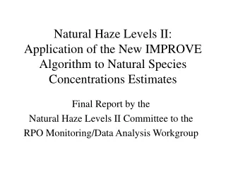
Update on Natural Levels II Technical Review Committee By Marc Pitchford for the June 12th RPO Monitoring/Data Analysis Conference Call
Overall Objective: • To agree on a methodology that estimates the worst and best natural conditions for each monitoring site for use with current conditions estimated by the new IMPROVE algorithm so that Regional Haze Rule glide paths can be calculated in a consistent way for states that wish to use the new algorithm.
Concerns Raised: • The new IMPROVE algorithm uses concentrations in an empirical approach to determine how much of the sulfate, nitrate, and organic concentrations should be in the large and small size distributions. We should assume that natural conditions have both large and small size distributions in about the same frequency but with (possibly) much lower concentrations. • All components of aerosol extinction should be scaled to Trijonis' natural values in a consistent manner. • Use of the baseline (2000 to 2004) to estimate site specific haze distribution functions (i.e. the standard distributions) on a site by site basis is liable to give distortions because one of the years had very unusual fire impacts at a number of western sites thereby giving a false sense of the width of the distributions. • We should check that the best day natural haze estimates at each site are consistent with the current best days (i.e. they shouldn't be larger than current best days).
Further modifications to natural condition estimates • Use scattering efficiencies as prescribed by the new IMPROVE algorithm • natural scenario “N” • Test the effect of basing natural mass concentrations on current values. • Assume 80% of current OMC is natural • Test the effect of using current OMC, EC, fine soil, and CM on G90 dv natural estimates • Look at the difference between current mean mass concentrations and naturals estimates by aerosol species
Scenarios where individual aerosol species mass is adjusted from natural estimates to current levels • N – uses Trijonis east/west mass concentrations • N1 – scale only SO4 and NO3 to estimated natural mass concentrations (presentation 5) • N2 – scale only SO4, NO3 and EC to estimated natural mass concentrations (presentation 5) • N3 – OMC adjusted to 80% of current mean • N4 – OMC = current mean • N5 – EC = current mean • N6 – fine soil = current mean • N7 – coarse mass = current mean • N8 – fine soil and CM = current mean • Sensitivities of scenario N to scenarios N3…N8 • Mass adjustments (current to natural estimate mean mass shifts)
Scale aerosol mass frequency distributions Current 2000-2004 Hanging bars Solid - current mean Dashed - natural estimate mean • Sipsey Alabama • Each aerosol species mass concentration frequency distribution scaled to estimated natural mass concentrations • If current species mean is less than natural estimate, the that species is not scaled • Geometric shape of species distributions is unchanged Natural Estimate
Scaled aerosol extinction distributions Current 2000-2004 Hanging bars Solid - current mean Dashed - natural estimate mean • Sipsey Alabama • For SO4, NO3 and OMC use the current daily scattering efficiencies to calculate species extinction (scenario Nb) • Joint aerosol extinction frequency distribution shape is altered from the current distribution Natural Estimate
Aerosol bext and dv frequency distributions current and scenario Nb • Sipsey Alabama • Natural scenario joint distribution shape is derived from scaling current aerosol species mass concentrations to natural condition estimates • Allows estimation of worst 20% dv or aerosol species extinction
Scenario N G90 dv • All species adjusted to natural estimate east/west mean mass concentrations
Scenario N3 G90 dv • All species except OMC adjusted to natural estimate east/west means • OMC adjusted to 80% of current mean
Scenario N4 G90 dv • All species except OMC adjusted to natural estimate east/west means • OMC = current mean
Scenario N5 G90 dv • All species except EC adjusted to natural estimate east/west means • EC = current mean
Scenario N6 G90 dv • All species except fine soil adjusted to natural estimate east/west means • fine soil = current mean
Scenario N7 G90 dv • All species except CM adjusted to natural estimate east/west mean • CM = current mean
Scenario N8 G90 dv • All species except fine soil and CM adjusted to natural estimate east/west mean • Fine soil and CM = current mean
Sensitivity of G90 dv: scenario N to N3 • G90 dv change – increase OMC from natural estimate to 80% of current levels
Sensitivity of G90 dv: scenario N to N4 • G90 dv change – increase OMC from natural estimate to current levels
Sensitivity of G90 dv: scenario N to N5 • G90 dv change – increase EC from natural estimate to current levels
Sensitivity of G90 dv: scenario N to N6 • G90 dv change – increase fine soil from natural estimate to current levels
Sensitivity of G90 dv: scenario N to N7 • G90 dv change – increase CM from natural estimate to current levels
Sensitivity of G90 dv: scenario N to N8 • G90 dv change – increase CM and Soil from natural estimates to current levels
5-yr baseline vs. long-term estimatesscenario Nb Difference in worst 20% dv natural estimate 2000-2004 1988-2004
Status/Next Steps • Status: • The “N” approach (current baseline values scaled to Trijonis average natural species concentrations and using the new algorithm extinction without adjustments) is the most defensible of the approaches tried. • The use of current (or 80% of current) OMC as natural may be justifiable for many sites, but is beyond the committee’s purview and time frame. • Next Steps: • Present material to larger audience • Document it for further dissemination and review
Appendix Maps of the difference between current species concentrations and natural levels.
aSO4: mass adjustment (Current – natural estimate) mean mass concentration difference
aNO3: mass adjustment (Current – natural estimate) mean mass concentration difference
OMC: mass adjustment (Current – natural estimate) mean mass concentration difference
EC: mass adjustment (Current – natural estimate) mean mass concentration difference
Soil: mass concentration adjustment (Current – natural estimate) mean mass concentration difference
CM: mass adjustment (Current – natural estimate) mean mass concentration difference
Sea Salt: mass adjustment (Current – natural estimate) mean mass concentration difference