Download
1 / 14
140 likes | 263 Views
Lecture 15: . Univariate Descriptive Statistics. Agenda. Finding Data for Quantitative Analysis Using Descriptive Statistics. Finding Data for Quantitative Analysis. Berkeley Survey Research Center http://srcweb.berkeley.edu/ UC Data (access to ICPSR) http://ucdata.berkeley.edu

E N D
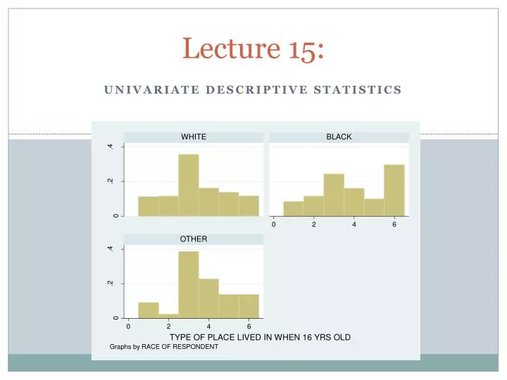
Lecture 15: Univariate Descriptive Statistics
Agenda • Finding Data for Quantitative Analysis • Using Descriptive Statistics
Finding Data for Quantitative Analysis • Berkeley Survey Research Center • http://srcweb.berkeley.edu/ • UC Data (access to ICPSR) • http://ucdata.berkeley.edu • Data on the Net • http://3stages.org/idata/
Probability and Statistics • Statistics deal with what we observe and how it compares to what might be expected by chance. • A set of probabilities corresponding to each possible value of some variable, X, creates a probability distribution • For now, we especially care about the normal (Gaussian) distribution
Describing Simple Distributions of Data • Central Tendency • Some way of “typifying” a distribution of values, scores, etc. • Mean (sum of scores divided by number of scores) • Median (middle score, as found by rank) • Mode (most common value from set of values) • In a normal distribution, all 3 measures are equal. • Example: GSS data
Special Features of the Mean • Sum of the deviations from the mean of all scores = zero. • Unlike the median, it is the point in a distribution where the two halves are balanced.
Using Central Tendencies in Recoding • “splitting” metrics into binary variables • “collapsing” variables
Dispersion • Range • Difference between highest value and the lowest value. • Standard Deviation • A statistic that describes how tightly the values are clustered around the mean. • Variance • A measure of how much spread a distribution has. • Computed as the average squared deviation of each value from its mean
Properties of Standard Deviation • Variance is just the square of the S.D. (or, S.D is the square root of the variance) • If a constant is added to all scores, it has no impact on S.D. • If a constant is multiplied to all scores, it will affect the dispersion (S.D. and variance) S = standard deviationX = individual scoreM = mean of all scoresn = sample size (number of scores)
Why Variance Matters… • In many ways, this is the purpose of many statistical tests: explaining the variance in a dependent variable through one or more independent variables.
Common Data Representations • Histograms • Simple graphs of the frequency of groups of scores. • Stem-and-Leaf Displays • Another way of displaying dispersion, particularly useful when you do not have large amounts of data. • Box Plots • Yet another way of displaying dispersion. Boxes show 75th and 25th percentile range, line within box shows median, and “whiskers” show the range of values (min and max)