Download

1 / 51
540 likes | 821 Views
Max Flow. Jose Rolim University of Geneva. Graph Models. Graphs (used as models of "transportation" networks) have the following components: Links / edges: carrier of some sort of traffic and have capacities Nodes: - source nodes: generate traffic

E N D
Max Flow Jose Rolim University of Geneva
Graph Models Graphs (used as models of "transportation" networks) have the following components: • Links / edges: carrier of some sort of traffic and have capacities • Nodes:- source nodes: generate traffic - sink nodes: absorb/demand traffic- intermediate nodes: "switches" which pass traffic between different edges • Description of the traffic itself Jose Rolim
Examples Jose Rolim
Example Graph - Sink node Source node Max. capacity of edge Actual flow through this edge Jose Rolim
Simplified Model The network is modeled simply as • a directed graph G = (V,E) with • non-negative capacity on each edge, • a single source node, s, and • a single sink node, t Jose Rolim
Some assumptions… We will simplify our discussion by assuming the following: • No edge enters s, the source • No edge leaves t, the sink • At least one edge is incident to each node • All capacities are integers Jose Rolim
Definition of Flow Flow will be our abstract term for the traffic; as an entity originating at the source node and absorbed at the sink node An (s,t) flow is a function f that assigns a non-negative number to each edge e in the graph G = (V,E) The value of a flow is Jose Rolim
Intuitive definition f(e) intuitively is the “flow” on edge e subject to two conditions: (i) capacity constraint: 0 ≤ f(e) ≤ c(e), where c(e) is the capacity of edge e (ii) conservation property: for each node v, other than s and t, ∑ f(e) = ∑ f(e) e into v v into e Jose Rolim
Max Flow Problem What is the maximum amount of flow that can be sustained in G? Clearly, the only obstacle to the flow are the capacities of the edges in G. The bottleneck doesn’t necessarily occur from the edges originating at s, or those terminating at t. It can arise from a complicated interaction among the edges, as flow snakes through G. Jose Rolim
Max Flow Problem Given a flow network G = (V,E,c), a source s, and a sink t, (1) What is the max flow that can be sustained in G (between s and t)? (2) Then, find an algorithm to best assign f values to the edges in G to answer (1) Jose Rolim
Sample Applications • The Max Flow problem shows up in many places, some less intuitive than others. • For instance, consider a shipping company seeking to ship as many units of a product (hockey pucks) as possible • Product starts at a source factory in Vancouver and ends in Winnipeg • The problem may be represented graphically as show in the following slide… Jose Rolim
Transportation (1). Let the capacity of an edge be the number of units that can be shipped between two cities by a shipping company (2). Let the current number of units being shipped between cities be denoted as flow between those cities. The following graph can therefore represent the problem: Nodes denote cities Can be interpreted as 4 units being shipped out of 4 possible Jose Rolim
Matrix Rounding A p x q matrix of decimals may be summed along the rows and columns Rounding each entry up or down between ceil(a) andfloor(a) may cause the sums to change. Trying to keep the sum consistent along rows does not necessarily keep the sum consistent along cols and vice-versa (see fig.) Jose Rolim
Max Flow as a Solution (1). Create a node, i, for each row, and a node, j, for each col in the matrix, and two additional nodes, s (source) and t (sink) (2). For each entry in the matrix, create an edge with cost (floor(Mij), ceil(Mij)) corresponding to rounding up or rounding down (3). Consistent matrix rounding is evidenced by feasible flow through the network Jose Rolim
Graph Representation (3,4) 1 1’ (6,7) (17,18) (7,8) (16,17) (9,10) (10,11) (12,13) (2,3) t 2 2’ s (0,1) (11,12) (14,15) (3,4) (1,2) 3 3’ (6,7) Jose Rolim
Scheduling • Assume a set of jobs, J, is to scheduled on M identical processors, with each job having 3 parameters: processing time (pi), ready time (ri) and due time (di). • ri+ pi<= diif the job can be performed • Preemption is allowed – jobs can be interrupted and restarted arbitrarily Jose Rolim
Example Let M = 3 for the following job set: The job set may therefore be represented graphically as shown Jose Rolim
Converting to Graph Form (1). Create a node for every interval in the interval diagram and one for every job as well as a source node, s, and a sink, t. (2). Connect s to job j with capacity pi. (3). Connect each interval node Tjkto sink t with capacity (k − j) * M, indicating the number of machine units available in that interval. (4). Connect a job i to each interval Tjksuch that ri % j and di ! k. The capacity of this edge is (k − j) indicating the number of machine units allotable to job i in this interval. (5). There is a soln to the problem iff there is a max flow of value Jose Rolim
Sample Graph This sample graph demonstrates some of the power of max flow. Many scheduling problems are NP-Complete, so finding a soln. to such a problem is very useful Thus max flow may be used to solve a wide range of seemingly unrelated problems and is useful beyond simple representations of computer networks Jose Rolim
Ford-Fulkerson Method • Developed by Ford and Fulkerson [1956] • Widely used and influential ideas: augmentation, residual network, and famous min-cut max-flow theorem. • Algorithm: Generic FF (G,s,t) • Initialize f = 0 (i.e. zero flow on all edges) • While there exists an “augmenting path” p from s to t • Push flow along p • Reduce capacities along p Jose Rolim
4 u v 2 5 6 5 t s 1 4 3 x y 2 Example 1: • According to the greedy approach of the Generic FF algorithm, consider the maximum flows from s to t. Jose Rolim
2/4 u v 2/2 2/5 t s Example 1 (contd.) • Path s-u-v-t gives f=2. Jose Rolim
t s 2/4 2/3 x y 2/2 Example 1 (contd.) • Path s-x-y-t gives f=2+2=4. Jose Rolim
4/4 u v 4/5 2/6 t s 4/4 x Example 1 (contd.) • Path s-x-u-v-t gives f=2+2+2=6. This gives us a total flow of 6, but it is not an optimal solution. Jose Rolim
Example 2: • By employing a greedy approach, we get a flow of 2. However, by not employing a greedy approach we can get a flow capacity of 3 in the above network. Jose Rolim
6/10 u v Residual Network • Given an edge (u,v) with residual capacity cf(u,v) of an edge (u,v) is defined as cf(u,v) = c(u,v) – f(u,v) • Residual capacity is the additional flow one can send on an edge, possibly by canceling some flow in opposite edge. • Example 1: cf(u,v) = 10-6 = 4 cf(u,v) = 0 - (- 6) = 6 Jose Rolim
Residual network • Residual network Gf is (V,Ef ), where Ef = {(u, v) | cf (u, v) > 0}. • Note: |Ef | <= 2|E|. • When is an edge (u, v) ε Ef? • if (u, v) ε E and f(u, v) < c(u, v), or • if (v, u) ε E and f(v, u) > 0. Jose Rolim
Example 2 Jose Rolim
Augmenting Paths • An augmenting path ‘p’ is a simple path in Gf from s to t. • The residual capacity of p is cf(p) = min { cf(u,v) | (u,v) ε p }. By definition, cf(p) > 0. • Can you spot an augmenting path in the graph below? Jose Rolim
1 u v 2 2 1 t s 1 1 1 x y 1 Example 1 Now, Ford-Fulkerson changes to – • Initialize f = 0 • While there exists an “augmenting path” p from s to t in Gf • Push flow along p • Reduce capacities along p Jose Rolim
t s 1 1 x y 1 Example 1(contd.) • Consider s-x-y-t • f = 1 Jose Rolim
1 u v 1 1 t s Example 1(contd.) • Consider s-u-v-t • f=1+1 Jose Rolim
1 u v 1 1 1 1 1 t s 1 1 1 x y 1 Example 1(contd.) • This gives us the intermediate graph: Jose Rolim
1 u v 2 2 1 1 t s 1 1 1 x y 1 Example 1(contd.) • Finally, considering s-u-y-x-v-t, we get the residual graph shown below. • f=1+1+1 = 3 Jose Rolim
Cuts • A cut (S, T) is a partition of V with s ε S and t ε T. • f(S, T) is the net flow across cut (S, T). • c(S, T) is the max capacity of cut (S, T); use only forward edges. Jose Rolim
Example 1 • In this example, f(S, T) = 12 − 4 + 11 = 19. • c(S, T) = 12 + 14 = 26. Jose Rolim
Flows and Cuts • No matter how you separate s and t, the net flow across (S, T) is exactly |f|. • Cut Lemma: If f is a flow and (S, T) a cut in G, then f(S, T) = |f|. Jose Rolim
Proof Jose Rolim
MaxFlow-MinCut Theorem • The following are equivalent: • f is a maxflow. • No augmenting path in Gf . • |f| = c(S, T) for some cut (S, T). PROOF: • (1) => (2). Augmenting path increases f. • (3) => (1). By Cut Lemma, |f| = f(S, T) ≤ c(S, T). So, equality means flow is a maxflow. • (2) => (3). • Define reachable set, S = {v | such that path from s to v in Gf} • T = V − S. Then, t ε T—because no augmenting path. For any u ε S, v ε T, • f(u, v) = c(u, v); otherwise, (u, v) ε Ef , and v will be reachable from s. • Thus, |f| = f(S, T) = c(S, T). Jose Rolim
Updated FF Algorithm • for each edge (u, v) єE do • f(u, v) = f(v, u) = 0; • while there is a path p in Gf do • cf (p) = min{cf (u, v) | (u, v) єp} • for each (u, v) єp do • f(u, v) = f(u, v) + cf (p) • f(v, u) = −f(u, v) • end • end. Jose Rolim
12 u v 16 20 4 t s 10 9 7 13 4 x y 14 Example 1 • Original Residual Graph • Choose a path Jose Rolim
12 u v 12 20 4 t s 14 9 7 13 4 4 x y 10 Example 1 (contd.) • Edit the path following the while loop • Choose a new path Jose Rolim
12 u v 12 13 4 7 t s 14 9 7 6 7 11 4 x y 3 Example 1 (contd.) • Keep iterating the while loop • Choose the final path Jose Rolim
12 u v 1 16 19 t s 14 9 7 6 7 11 4 x y 3 Example 1 (contd.) • No more augmenting paths • Final residual graph Jose Rolim
12/12 u v 16/16 19/20 4/4 t s 0/10 0/9 7/7 7/13 4/4 x y 11/14 Example 1 (contd.) • Final Capacity Graph • All (S,T) cuts = 23 Jose Rolim
Analysis of Ford - Fulkerson • Correctness follows from maxflow–mincut • BFS or DFS to find augmenting path takes O(m) time • If edge capacities are integers with maximum cap U, then the number of augmentations is at most Un • Total running time • O(m) * O(nU) = O(nmU) • If the edge capacities are irrational, then it is not clear that the algorithm will terminate in polynomial time. Jose Rolim
A Pathological Case for FF • For large edge capacities and certain graph topologies the run-time may be pathological. Assume M >109: Jose Rolim
Polynomial Time Maxflow • FF method does not prescribe how to pick augmenting paths • Edmunds-Karp heuristics: • Shortest augmenting path first • Max capacity augmentation • Heuristics are somewhat obvious, cleverness lies in their analysis Jose Rolim
Shortest Path Augmentation • Always augments flow from the shortest path from s to t • Let df(s, v) denote the shortest path distance from s to v in the current residual graph Gf . • Standard BFS algorithm finds the df(s, v) in O(m) time Jose Rolim
Shortest Path Augmentation Jose Rolim