Download
1 / 91
1.45k likes | 2.52k Views
MATLAB and Octave. An Introduction . INTRODUCTION. Octave and MATLAB are high-level languages, primarily intended for numerical computations. They provide a convenient command line interface for solving linear and nonlinear problems numerically.

E N D
MATLAB and Octave An Introduction
INTRODUCTION • Octave and MATLAB are high-level languages, primarily intended for numerical computations. • They provide a convenient command line interface for solving linear and nonlinear problems numerically. • They can also be used for prototyping and performing other numerical experiments.
Octave • MATLAB is a proprietary product that requires a license. • Octave is freely redistributable software. You may redistribute it and/or modify it under the terms of the GNU General Public License as published by the Free Software Foundation. • This document corresponds to Octave version 2.0.13.
Starting Octave • To start Octave type the shell command octave. You see a message then a prompt: octave:1> • If you get into trouble, you can usually interrupt octave by typing Ctrl-C to return to the prompt. • To exit Octave, type quit or exit at the prompt.
Creating a matrix • To create a new matrix and store it in a variable, type the command: octave:1> A=[1,1,2;3,5,8;13,21,34] • Octave will respond by printing the matrix in neatly aligned columns. 1 1 2 3 5 8 13 21 34
Controlling matrix output • Ending a command with a semicolon tells Octave to not print the result of a command. octave:2> B=rand(3,2); • will create a 3 row, 2 column matrix with each element set to a random value between zero and one. • To display the value of any variable, simply type the name of the variable. octave:3> B
Matrix arithmetic • Octave has a convenient operator notation for performing matrix arithmetic. To multiply the matrix a by a scalar, type: octave:4> 2*A • To multiply the two matrices A and B, type: octave:5> A*B • To form the matrix product type: octave:6> A’*A
Solving linear equations • To solve the set of linear equations Ax=b, use the left division operator \ : octave:7> A\b • This is conceptually equivalent to inverting the A matrix but avoids computing the inverse of a matrix directly. • If the coefficient matrix is singular, Octave will print a warning message.
Graphical output • To display an x-y plot, use the command: octave:8> plot(x,sin(x)) • If you are using the X Window System, Octave will automatically create a separate window to display the plot. • Octave uses gnuplot to display graphics, and can display graphics on any terminal that is supported by gnuplot.
Getting hardcopy • To capture the output of the plot command in a file rather than sending the output directly to your terminal, you can use a set of commands like this: gset term postscript gset output "foo.ps" replot • This will work for other types of output devices as well.
DATA TYPES • The standard built-in data types are • real and complex scalars, • real and complex matrices, • ranges, • character strings, • a data structure type.
Numeric data objects • All built-in numeric data is currently stored as double precision numbers. • On systems that use the IEEE floating point format, values in the range of approximately 1.80e+308to 2.23e-308 can be stored, and the relative precision is approximately 2.22e-16. • The exact values are given by the variables realmin,realmax and eps respectively.
Matrix objects • Matrix objects can be of any size, and can be dynamically reshaped and resized. • It is easy to extract: • rows, A(i,:) selects the ith row of the matrix, • columns , A(:,j) selects thejth column of the matrix, or • sub-matrices, A([i1:i2],[j1:j2]) selects rows i1 to i2and columnsj1 toj2.
Range objects • A range expression is defined by the value of the first element in the range, an optional value for the increment between elements, and a maximum value which the elements of the range will not exceed. • The base, increment, and limit are separated by colons and may contain any arithmetic expressions and function calls.
String objects • A character string in Octave consists of a sequence of characters enclosed in either double-quote or single-quote marks. • Internally, Octave currently stores strings as matrices of characters. • All the indexing operations that work for matrix objects also work for strings.
Data structure objects • Octave's data structure type can help you to organize related objects of different types. • The current implementation uses an associative array with indices limited to strings x.a=1 x.b=[1,2;3,4] x.c="string" creates a structure with three elements.
Object sizes • A group of functions allow you to display the size of a variable or expression. • These functions are defined for all objects. They return -1 when the operation doesn't make sense. • For example, the data structure type doesn't have rows or columns, so the rows and columns functions return -1 for structure arguments.
Object size functions • columns(A) • Return the number of columns of A. • rows(A) • Return the number of rows of A. • length(A) • Return the number of rows of A or the number of columns ofA, whichever is larger.
More object size functions • d=size(A) • Return the number rows and columns of A, the result is returned in the 2 element row vector d. • [nr,nc]=size(A) • The number of rows is assigned to nr and the number of columns is assigned to nc. • d=size(A,n) • A second argument of either n=1 or n=2, size will return only the row or column dimension.
Detecting object properties • is_matrix(A) • Return 1 if A is a matrix. Otherwise, return 0. • is_vector(A) • Return 1 if A is a vector. Otherwise, return 0. • is_scalar(A) • Return 1 if A is a scalar. Otherwise, return 0.
Detecting matrix properties • is_square(A) • If A is a square matrix, then return the dimension of A. Otherwise, return 0. • is_symmetric(A,tol) • If A is symmetric within the tolerance specified , then return the dimension of A. Otherwise, return 0. If tol is omitted, tol=eps • isempty(A) • If A is empty return 1. Otherwise, return 0.
Range definition • The range 1:5 • defines the set of values [1,2,3,4,5]. • The range 1:2:5 • defines the set of values [1,3,5]. • The range 1:3:5 • defines the set of values [1,4]. • The range 5:-3:1 • defines the set of values [5,2].
More about ranges • Note that the upper (or lower, if the increment is negative) bound on the range is not always included in the set of values. • Ranges defined by floating point values can produce surprising results because floating point arithmetic is used. • If it is important to include the endpoints of a range and the number of elements is known, use the linspace() function.
Special matrix object eye() • eye(x) • If invoked with a single scalar argument, eye returns a square identity matrix with the dimension specified. • eye(n,m) or eye(size(A)) • If you supply two scalar arguments, eye takes them to be the number of rows and columns. • eye • Calling eye with no arguments is equivalent to calling it with an argument of 1.
Special matrix object ones() • ones(x) • If invoked with a single scalar argument, ones returns a square matrix of 1’s with the dimension specified. • ones(n,m) or ones(size(A)) • If you supply two scalar arguments, ones takes them to be the number of rows and columns. • ones • Calling ones with no arguments is equivalent to calling it with an argument of 1.
Special matrix object zeros() • zeros(x) • If invoked with a single scalar argument, zeros returns a square matrix of 0’s with the dimension specified. • zeros(n,m) or zeros(size(A)) • If you supply two scalar arguments, zeros takes them to be the number of rows and columns. • zeros • Calling zeros with no arguments is equivalent to calling it with an argument of 1.
Special matrix object rand() • rand(x) • If invoked with a single scalar argument, rand returns a square matrix of random numbers between 0 and 1 with the dimension specified. • rand(n,m) or rand(size(A)) • If you supply two scalar arguments, rand takes them to be the number of rows and columns. • rand • Calling rand with no arguments is equivalent to calling it with an argument of 1.
Special matrix object randn() • randn(x) • With a single scalar argument, randn returns a square matrix of Gaussian random numbers between 0 and 1 with the dimension specified. • randn(n,m) or randn(size(A)) • For two scalar arguments, randn takes them to be the number of rows and columns. • randn • Calling rand with no arguments is equivalent to calling it with an argument of 1.
Random number seeds • Normally, randand randn obtain their initial seeds from the system clock,so that the sequence of random numbers is not the same each time you run Octave. • To allow generation of identical sequences, rand and randn allow the random number seed to be specified. rand(‘seed’,value) or randn(‘seed’,value)
STRINGS • A string constant consists of a sequence of characters enclosed in either double-quote or single-quote marks: • Strings in Octave can be of any length. • Since the single-quote mark is also used for the transpose operator it is best to use double-quote marks to denote strings.
Literals • Some characters cannot be included literally in a string constant. You represent them instead with escape sequences, which are character sequences beginning with a backslash ( \ ). • Another use of backslash is to represent unprintable characters such as newline \n or tab \t and others.
String functions • blanks(n)Return a string of n blanks. • setstr(A)Convert a matrix to a string. Each numeric element is converted to an ascii character. • strcat(s1,...,sn)Return a string containing all the arguments concatenated. • str2mat(s1,..., sn)Return a valid string matrix containing the strings s1, ..., sn as its rows. • deblank(s)Removes the trailing blanks from the string s.
String comparison • index(s1,s2)Return the position of the first occurrence of the string s2 in s1, or 0 if not found. Note: index does not work for arrays of strings. • rindex(s1,s2)Return the position of the last occurrence of the string s2 in s1, or 0 if not found. Note: rindex does not work for arrays of strings. • strcmp(s1,s2)Compares two strings, return 1 if they are the same, otherwise 0. • isstr(s)Return 1 if s is a string, otherwise, 0.
Substring functions • findstr(s1,s2)Return the vector of all positions in the longer string where an occurrence of the shorter substring starts. • split(s1,s2)Divide s1 into substrings separated by s2, returning a valid string array. • strrep(s1,s2,s3)In string s1, replace all occurrences of the substring s2 with substring s3. • substr(s,n1,n2)Return the substring of s starting at character n1 and is n2 characters long.
String conversions • bin2dec(s)Return a decimal number corresponding to the binary number represented as a string of 0s and 1s. • dec2bin(n)Return a binary number as a string of 0s and 1s corresponding the non-negative decimal number n. • hex2dec(s)Return a decimal number corresponding to the hexadecimal number stored in the string s. • dec2hex(n)Return the hex number corresponding to the non-negative decimal number n, as a string. • str2num(s)Convert the string s to a number. • num2str(n)Convert the number n to a string.
More string conversions • toascii(s)Return ascii representation of s in a matrix. • tolower(s)Return a copy of the string s, with each upper-case character replaced by the corresponding lower-case one; non-alphabetic characters are left unchanged. • toupper(s)Return a copy of the string s, with each lower-case character replaced by the corresponding upper-case one; non-alphabetic characters are left unchanged.
Testing characters • The above functions return 1 (true) or 0 (false) if the tested character is in the set represented by the function.
VARIABLES • Variables let you give names to values and refer to them later. • The name of an Octave variable must be a sequence of letters, digits and underscores, but it may not begin with a digit. • There is no limit on the number of characters in a variable name. • Case is significant in variable names. The symbolsa and A are distinct variables.
Built-in variables • A number of variables have special built-in meanings. For example, PWD holds the current working directory, and pi names the ratio of the circumference of a circle to its diameter. • Octave has a long list of all the predefined variables. Some of these built-in symbols are constants and may not be changed.
Status of variables • clear options pattern Delete the names matching the given patterns from the symbol table. • who options pattern • whos options pattern List currently defined symbols matching the given patterns.
Options The following are valid options for the clear and who functions. They may be shortened to one character but may not be combined. • -a(ll) List all currently defined symbols. • -b(uiltins) List built-in variables and functions. • -f(unctions) List user-defined functions. • -l(ong) Print a long listing of symbols • -v(ariables) List user-defined variables.
EXPRESSIONS • Expressions are the basic building block of statements in Octave. • An expression evaluates to a value, which you can print, test, store in a variable, pass to a function, or assign a new value to a variable with an assignment operator. • An expression alone can serve as a statement. Most statements contain one or more expressions which specify data to be operated on. • Expressions include variables, array references, constants, and function calls, as well as combinations of these with various operators.
Index expressions • An index expression allows you to reference or extract selected elements of a matrix or vector. • Indices may be scalars, vectors, ranges, or the special operator ( : ) ,which may be used to select entire rows or columns. • A(i,:) • A(:,j) • A(i1:i2,j1:j2)
Addition operators • x+y • Addition. If both operands are matrices, the number of rows and columns must both agree. • x.+y • Element by element addition. This is equivalent to the + operator. • x-y • Subtraction. If both operands are matrices, the number of rows and columns of both must agree. • x.-y • Element by element subtraction. This is equivalent to the - operator.
Multiplication operators • x*y • Matrix multiplication. The number of columns of x must agree with the number of rows of y. • x.*y • Element by element multiplication. If both operands are matrices, the number of rows and columns must both agree.
Division operators • x/y • Right division. Equivalent to(inv(y')*x')' • x./y • Element by element right division. Each element of x is divided by each corresponding element of y. • x\y • Left division. Equivalent to the inv(x)*y • x.\y • Element by element left division. Each element of y is divided by each corresponding element of x.
Power operators • x^y or x**y • Power operator. • x and y both scalar: returns x raised to the power y. • x scalar, y is a square matrix : returns result using eigenvalue expansion. • x is a square matrix and y scalar: returns result by repeated multiplication if y is an integer, else by eigenvalue expansion. • x and y both matrices: returns an error. • x.^y or x.**y • Element by element power operator. • If both operands are matrices, the number of rows and columns must both agree.
Unary operators • +x or +x. • A unary plus operator has no effect on the operand. • -x or -x. • Negation or element by element negation. • x' • Complex conjugate transpose. For real arguments, this is the same as the transpose operator. For complex arguments, equivalent to conj(x.') • x.' • Element by element transpose.
Comparison operators • Comparison operators compare numeric values for relationships. • All of comparison operators return a value of 1 if the comparison is true, or 0 if it is false. • For matrix values, the comparison is on an element-by-element basis. • [1,2;3,4]==[1,3;2,4];ans=[1,0;0,1] • For mixed scalar and matrix operands, the scalar is compared to each element in turn. • [1,2;3,4]==2;ans=[0,1;0,0]
Relational operators • x<y True if x is less than y. • x<=yTrue if x is less than or equal to y. • x==yTrue if x is equal to y. • x>=yTrue if x is greater than or equal to y. • x>yTrue if x is greater than y. • x!=y True if x is not equal to y. • x~=yTrue if x is not equal to y. • x<>yTrue if x is not equal to y.