Software Representation of the ATLAS Solenoid Magnetic Field

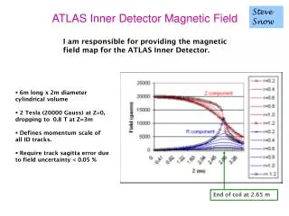
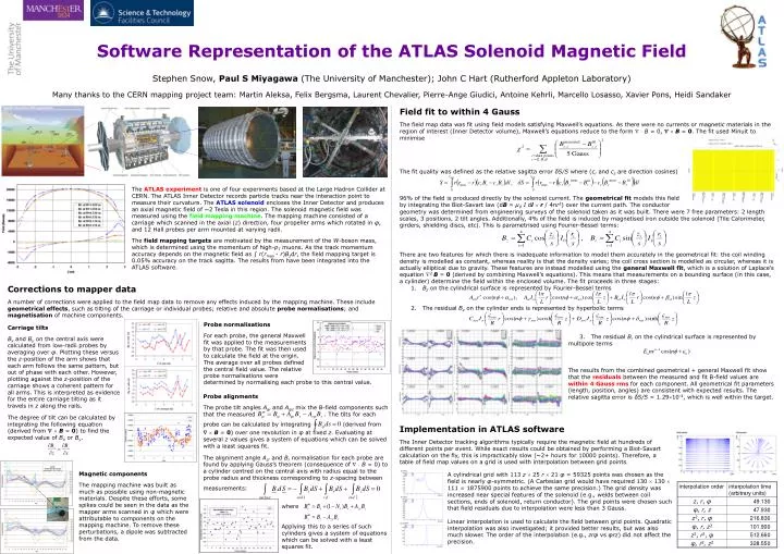
1. Software Representation of the ATLAS Solenoid Magnetic Field Stephen Snow, Paul S Miyagawa (The University of Manchester); John C Hart (Rutherford Appleton Laboratory)Many thanks to the CERN mapping project team: Martin Aleksa, Felix Bergsma, Laurent Chevalier, Pierre-Ange Giudici, Antoine Kehrli, Marcello Losasso, Xavier Pons, Heidi Sandaker Field fit to within 4 GaussThe field map data was fit using field models satisfying Maxwell’s equations. As there were no currents or magnetic materials in the region of interest (Inner Detector volume), Maxwell’s equations reduce to the form   B = 0,   B= 0. The fit used Minuit to minimiseThe fit quality was defined as the relative sagitta error δS/S where (crand czare direction cosines) The ATLAS experiment is one of four experiments based at the Large Hadron Collider at CERN. The ATLAS Inner Detector records particle tracks near the interaction point to measure their curvature. The ATLAS solenoidencloses the Inner Detector and produces an axial magnetic field of ~2 Tesla in this region. The solenoid magnetic field was measured using the field mapping machine. The mapping machine consisted of a carriage which scanned in the axial (z) direction, four propeller arms which rotated in φ, and 12 Hall probes per arm mounted at varying radii.The field mapping targets are motivated by the measurement of the W-boson mass, which is determined using the momentum of high-pT muons. As the track momentum accuracy depends on the magnetic field as ∫r(rmax - r)Bzdr, the field mapping target is 0.05% accuracy on the track sagitta. The results from have been integrated into the ATLAS software. 96% of the field is produced directly by the solenoid current. The geometrical fit models this field by integrating the Biot-Savart law (dB = μ0I dl r / 4πr3) over the current path. The conductor geometry was determined from engineering surveys of the solenoid taken as it was built. There were 7 free parameters: 2 length scales, 3 positions, 2 tilt angles. Additionally, 4% of the field is induced by magnetised iron outside the solenoid (Tile Calorimeter, girders, shielding discs, etc). This is parametrised using Fourier-Bessel terms: There are two features for which there is inadequate information to model them accurately in the geometrical fit: the coil winding density is modelled as constant, whereas reality is that the density varies; the coil cross section is modelled as circular, whereas it is actually elliptical due to gravity. These features are instead modelled using the general Maxwell fit, which is a solution of Laplace’s equation 2 B = 0 (derived by combining Maxwell’s equations). This means that measurements on a bounding surface (in this case, a cylinder) determine the field within the enclosed volume. The fit proceeds in three stages: 1. Bz on the cylindrical surface is represented by Fourier-Bessel terms 2. The residual Bz on the cylinder ends is represented by hyperbolic terms Corrections to mapper dataA number of corrections were applied to the field map data to remove any effects induced by the mapping machine. These include geometrical effects, such as tilting of the carriage or individual probes; relative and absolute probe normalisations; and magnetisation of machine components. Probe normalisationsFor each probe, the general Maxwell fit was applied to the measurements by that probe. The fit was then used to calculate the field at the origin. The average over all probes defined the central field value. The relative probe normalisations were Carriage tiltsBx and By on the central axis were calculated from low-radii probes by averaging over φ. Plotting these versus the z-position of the arm shows that each arm follows the same pattern, but out of phase with each other. However, plotting against the z-position of the carriage shows a coherent pattern for all arms. This is interpreted as evidence for the entire carriage tilting as it travels in z along the rails.The degree of tilt can be calculated by integrating the following equation (derived from   B= 0) to find the expected value of Bx or By. 3. The residual Br on the cylindrical surface is represented by multipole termsThe results from the combined geometrical + general Maxwell fit show that the residuals between the measured and fit B-field values are within 4 Gauss rms for each component. All geometrical fit parameters (length, position, angles) are consistent with expected results. The relative sagitta error is δS/S = 1.2910-4, which is well within the target. determined by normalising eachprobe to this central value. Probe alignmentsThe probe tilt angles Aφr and Aφzmix the B-field components such that the measured . The tilts for eachprobe can be calculated by integrating (derived from  B= 0) over one revolution in φ at fixed z. Evaluating at several z values gives a system of equations which can be solved with a least squares fit.The alignment angle Azr and Br normalisation for each probe are found by applying Gauss’s theorem (consequence of   B = 0) to a cylinder centred on the central axis with radius equal to the probe radius and thickness corresponding to z-spacing betweenmeasurements: Implementation in ATLAS softwareThe Inner Detector tracking algorithms typically require the magnetic field at hundreds of different points per event. While exact results could be obtained by performing a Biot-Savart calculation on the fly, this is impracticably slow (~2+ hours for 10000 points). Therefore, a table of field map values on a grid is used with interpolation between grid points. Magnetic componentsThe mapping machine was built as much as possible using non-magnetic materials. Despite these efforts, some spikes could be seen in the data as the mapper arms scanned in φ which were attributable to components on the mapping machine. To remove these perturbations, a dipole was subtracted from the data. A cylindrical grid with 113 z 25 r  21 φ = 59325 points was chosen as the field is nearly φ-symmetric. (A Cartesian grid would have required 130  130  111 = 1875900 points to achieve the same precision.) The grid density was increased near special features of the solenoid (e.g., welds between coil sections, ends of solenoid, return conductor). The grid points were chosen such that field residuals due to interpolation were less than 3 Gauss.Linear interpolation is used to calculate the field between grid points. Quadratic interpolation was also investigated; it provided better results, but was also much slower. The order of the interpolation (e.g., zrφ vs φrz) did not affect the precision. whereApplying this to a series of such cylinders gives a system of equations which can be solved with a least squares fit.