If we apply the Fokker-Planck analysis to geometric Brownian motion we get the equation

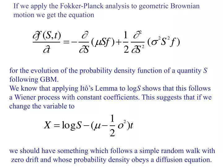
1. If we apply the Fokker-Planck analysis to geometric Brownian motion we get the equation for the evolution of the probability density function of a quantity S following GBM. We know that applying Itô’s Lemma to logS shows thatthis follows a Wiener process with constant coefficients. This suggests that if we change the variable to we should have something which follows a simple random walk with zero drift and whose probability density obeys a diffusion equation.

2. As argued before, the probability density function for X is related to that for S by since

3. Now, this gives and

4. Putting these together and using the F-P equation we get An initial value for f(S,0) on the domain (0,∞ ) can be converted into an expression for g(X,0) and the solution for f(S,t) found by transforming back the solution for g which we already know. This shows how a knowledge of the relation between the stochastic differential equations for f and g can lead us to the transformation needed to simplify this particular F-P equation. The Black-Scholes equation which describes option pricing will be seen in due course to be soluble using similar transformations.

5. A general remark on diffusion equations. The solution of the diffusion equation produces a spreading out and flattening of the initial profile and any small ripples on the profile disappear. If we try to start from the profile after some time and integrate backwards to get the initial condition then any small errors will grow and the problem is inherently unstable. The same holds if we try to integrate forward in time with a negative diffusion coefficient. The Black-Scholes equation contains a diffusion term with negative sign. However, in this case we need to integrate backwards in time. What we have is a known option value on the expiry date and we want to use this to obtain the value now.

6. In the simplest option pricing problem an analytic solution of the B-S equation can be found, but for more complicated financial derivatives numerical techniques may be necessary. Here we give a very brief outline of these. For simplicity we consider the simple diffusion equation Note that we can always make D unity by scaling the variables. Now consider a finite difference approximation where we take values of f on a grid x0 , x1 …….. at time intervals t. Let be the value at the mth time step at position xn .

7. The simplest approximation is just to take which gives Note that this gives a simple formula for the values at the next time in terms of those at the present time. Such a scheme is called an explicit scheme. Does it work?

8. This shows solutions with an initial triangular profile and x= 0.1, t=0.002

9. This seems to work, but the time step is very small. Suppose we increase it to 0.01, then we get the behaviour below, which is not a plausible looking solution of the diffusion equation. It is typical of explicit schemes that they go unstable unless the time step is small enough.

10. In order to follow the solution for a long time without using a ridiculously large number of time steps we go to an implicit scheme. A fully implicit scheme is similar to what we had before, but on the right hand side we use the values at time m+1. Then we obtain so we have to solve a set of linear equations to find the new values. The extra complication this entails is more than offset by the fact that this scheme is always stable. A time step which is too large may lead to loss of accuracy, but the whole solution will not go completely haywire as happens with an unstable scheme.

11. This shows the same problem as before, with a time step which would be unstable in an explicit scheme. A widely used variant of this is the Crank-Nicholson scheme where the rhs is taken to be the average of the explicit and implicit versions. This preserves stability and is more accurate than a simple implicit scheme.