Download
1 / 48
480 likes | 577 Views
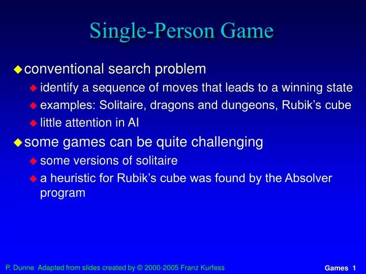
Single-Person Game. conventional search problem identify a sequence of moves that leads to a winning state examples: Solitaire, dragons and dungeons, Rubik’s cube little attention in AI some games can be quite challenging some versions of solitaire

E N D
Single-Person Game • conventional search problem • identify a sequence of moves that leads to a winning state • examples: Solitaire, dragons and dungeons, Rubik’s cube • little attention in AI • some games can be quite challenging • some versions of solitaire • a heuristic for Rubik’s cube was found by the Absolver program
Two-Person Game • games with two opposing players • often called MAXand MIN • usually MAX moves first, then min • in game terminology, a move comprises one step, or play by each player • Typically you are Max • MAX wants a strategy to find a winning state • no matter what MIN does • Max must assume MIN does the same • or at least tries to prevent MAX from winning
Perfect Decisions • Optimal strategy for MAX • traverse all relevant parts of the search tree • this must include possible moves by MIN • identify a path that leads MAX to a winning state • So MAX must do some work to estimate all the possible moves (to a certain depth) from the current position and try to plan the best way forward such that he will win • often impractical • time and space limitations
Nodes are discovered using DFS Once leaf nodes are discovered they are scored Here Max is building a tree of possibilities Which way should he play when the tree is finished? Max’s possible moves Mins’s possible moves Max’s moves Mins’s moves 4 7 9
Max-Min Example terminal nodes: values calculated from the utility function 4 7 9 6 9 8 8 5 6 7 5 2 3 2 5 4 9 3
MiniMax Example other nodes: values calculated via minimax algorithm Here the green nodes pick the minimum value from the nodes underneath 4 7 6 2 6 3 4 5 1 2 5 4 1 2 6 3 4 3 Min 4 7 9 6 9 8 8 5 6 7 5 2 3 2 5 4 9 3
MiniMax Example other nodes: values calculated via minimax algorithm Here the red nodes pick the maximum value from the nodes underneath 7 6 5 5 6 4 Max 4 7 6 2 6 3 4 5 1 2 5 4 1 2 6 3 4 3 Min 4 7 9 6 9 8 8 5 6 7 5 2 3 2 5 4 9 3
MiniMax Example other nodes: values calculated via minimax algorithm 5 3 4 Min 7 6 5 5 6 4 Max 4 7 6 2 6 3 4 5 1 2 5 4 1 2 6 3 4 3 Min 4 7 9 6 9 8 8 5 6 7 5 2 3 2 5 4 9 3
MiniMax Example 5 Max 5 3 4 Min 7 6 5 5 6 4 Max 4 7 6 2 6 3 4 5 1 2 5 4 1 2 6 3 4 3 Min 4 7 9 6 9 8 8 5 6 7 5 2 3 2 5 4 9 3
MiniMax Example 5 Max moves by Max and countermoves by Min 5 3 4 Min 7 6 5 5 6 4 Max 4 7 6 2 6 3 4 5 1 2 5 4 1 2 6 3 4 3 Min 4 7 9 6 9 8 8 5 6 7 5 2 3 2 5 4 9 3
MiniMax Observations • the values of some of the leaf nodes are irrelevant for decisions at the next level • this also holds for decisions at higher levels • as a consequence, under certain circumstances, some parts of the tree can be disregarded • it is possible to still make an optimal decision without considering those parts
What is pruning? • You don’t have to look at every node in the tree • discards parts of the search tree • That are guaranteed not to contain good moves • results in substantial time and space savings • as a consequence, longer sequences of moves can be explored • the leftover part of the task may still be exponential, however
Alpha-Beta Pruning • extension of the minimax approach • results in the same move as minimax, but with less overhead • prunes uninteresting parts of the search tree • certain moves are not considered • won’t result in a better evaluation value than a move further up in the tree • they would lead to a less desirable outcome • applies to moves by both players • a indicates the best choice for Max so far never decreases • b indicates the best choice for Min so far never increases
Note • For the following example remember: • Nodes are found with DFS • As a terminal or leaf node (or at a temporary terminal node at a certain depth) is found a utility function gives it a score • So do we need to evaluate F and G once we find E? Can we prune the tree? 5 E F G
Alpha-Beta Example 1 [-∞, +∞] 5 Max Local Values • Step 1 --- we expand the tree a little • we assume a depth-first, left-to-right search as basic strategy • the range ( [-∞, +∞] ) of the possible values for each node are indicated • initially the local values [-∞, +∞] reflect the values of the sub-trees in that node from Max’s or Min’s perspective; • Since we haven’t expanded they are infinite • the global values and are the best overall choices so far for Max or Min [-∞, +∞] Min • a best choice for Max ? • b best choice for Min ? Global Values
Alpha-Beta Example 2 [-∞, +∞] 5 Max • We evaluate a node • Min obtains the first value from a successor node [-∞, 7] Min 7 • a best choice for Max ? • b best choice for Min 7 @ min node if value of node < value of parent then abandon. …NO because no a yet
Alpha-Beta Example 3 [-∞, +∞] 5 Max • Min obtains the second value from a successor node [-∞, 6] Min 7 6 • a best choice for Max ? • b best choice for Min 6 @ min node if value of node < value of parent then abandon. …NO
Alpha-Beta Example 4 [5, +∞] 5 Max • Min obtains the third value from a successor node • this is the last value from this sub-tree, and the exact value is known • Min is finished on this branch • Max now has a value for its first successor node, but hopes that something better might still come 5 Min 7 6 5 • a best choice for Max 5 • b best choice for Min 5 @ min node if value of node < value of parent then abandon. …No more nodes
Alpha-Beta Example 5 [5, +∞] 5 Max • Min continues with the next sub-tree, and gets a better value • Max has a better choice from its perspective (the ‘5’) and should not consider a move into the sub-tree currently being explored by Min 5 [-∞, 3] Min 7 6 5 3 • a best choice for Max 5 • b best choice for Min 3 @ min node if value of node < value of parent then abandon. …YES!
Alpha-Beta Example 6 [5, +∞] 5 Max • Max won’t consider a move to this sub-tree it would choose 5 first =>abandon expansion • this is a case of pruning, indicated by • Pruning means that we won’t do a DFS into these nodes • No need to use the utility function to calculate the nodes value • No need to explore that part of the tree further. 5 [-∞, 3] Min 7 6 5 3 • a best choice for Max 5 • b best choice for Min 3 @ min node if value of node < value of parent then abandon. …YES!
Alpha-Beta Example 7 [5, +∞] 5 Max • Min explores the next sub-tree, and finds a value that is worse than the other nodes at this level • Min knows this ‘6’ is good for Max and will then evaluate the leaf nodes looking for a lower value (if it exists) • if Min is not able to find something lower, then Max will choose this branch 5 [-∞, 3] [-∞, 6] Min 7 6 5 3 6 • a best choice for Max 5 • b best choice for Min 3 @ min node if value of node < value of parent then abandon. …NO
Alpha-Beta Example 8 [5, +∞] 5 Max • Min is lucky, and finds a value that is the same as the current worst value at this level • Max can choose this branch, or the other branch with the same value 5 [-∞, 3] [-∞, 5] Min 7 6 5 3 6 5 • a best choice for Max 5 • b best choice for Min 3 @ min node if value of node < value of parent then abandon. …YES!
Alpha-Beta Example 9 5 5 Max • Min could continue searching this sub-tree to see if there is a value that is less than the current worst alternative in order to give Max as few choices as possible • this depends on the specific implementation • Max knows the best value for its sub-tree 5 [-∞, 3] [-∞, 5] Min 7 6 5 3 6 5 • a best choice for Max 5 • b best choice for Min 3
Properties of Alpha-Beta Pruning • in the ideal case, the best successor node is examined first • alpha-beta can look ahead twice as far as minimax • assumes an idealized tree model • uniform branching factor, path length • random distribution of leaf evaluation values • requires additional information for good players • game-specific background knowledge • empirical data
Imperfect Decisions • Does this mean I have to expand the tree all the way??? • complete search is impractical for most games • alternative: search the tree only to a certain depth • requires a cutoff-test to determine where to stop
Evaluation Function • If I stop part of the way down how do I score these nodes (which are not terminal nodes!) • Use an evaluation function to score these nodes! • must be consistent with the utility function • values for terminal nodes (or at least their order) must be the same • tradeoff between accuracy and time cost • without time limits, minimax could be used
Example: Tic-Tac-Toe • simple evaluation function E(s) = (rx + cx + dx) - (ro + co + do) where r,c,d are the number of rows, columns and diagonals lines available for a win for X (or O) in that state; x and o are the pieces of the two players • 1-ply lookahead • start at the top of the tree • evaluate all 9 choices for player 1 • pick the maximum E-value • 2-ply lookahead • also looks at the opponents possible move • assuming that the opponents picks the minimum E-value
Tic-Tac-Toe 1-Ply E(s0) = Max{E(s11), E(s1n)} = Max{2,3,4} = 4 E(s1:1) 8 - 5 = 3 E(s1:2) 8 - 6 = 2 E(s1:3) 8 - 5 = 3 E(s1:4) 8 - 6 = 2 E(s1:5) 8 - 4 = 4 E(s1:6) 8 - 6 = 2 E(s1:7) 8 - 5 = 3 E(s1:8) 8 - 6 = 2 E(s1:9) 8 - 5 = 3 X X X X X X X X X E(s1:1) == E of state @ depth-level ‘1’ number ‘1’ Simple evaluation function E(s1:1) = (rx + cx + dx) - (ro + co + do) E(s1:1) = ‘X’ has (3rows + 3 cols + 2 diags) – ‘O’ has (2r + 2c +1d) E(s11) = 8 -5 = 3
Tic-Tac-Toe 2-Ply E(s0) = Max{E(s11), E(s1n)} = Max{2,3,4} = 4 E(s1:1) 8 - 5 = 3 E(s1:2) 8 - 6 = 2 E(s1:3) 8 - 5 = 3 E(s1:4) 8 - 6 = 2 E(s1:5) 8 - 4 = 4 E(s1:6) 8 - 6 = 2 E(s1:7) 8 - 5 = 3 E(s1:8) 8 - 6 = 2 E(s1:9) 8 - 5 = 3 X X X X X X X X X E(s2:41) 5 - 4 = 1 E(s2:42) 6 - 4 = 2 E(s2:43) 5 - 4 = 1 E(s2:44) 6 - 4 = 2 E(s2:45) 6 - 4 = 2 E(s2:46) 5 - 4 = 1 E(s2:47) 6 - 4 = 2 E(s2:48) 5 - 4 = 1 O O O X X X O X X O X X X O O O E(s2:9) 5 - 6 = -1 E(s2:10) 5 -6 = -1 E(s2:11) 5 - 6 = -1 E(s2:12) 5 - 6 = -1 E(s2:13) 5 - 6 = -1 E(s2:14) 5 - 6 = -1 E(s2:15) 5 -6 = -1 E(s2:16) 5 - 6 = -1 O X X O X X X X X X O O O O O O E(s21) 6 - 5 = 1 E(s22) 5 - 5 = 0 E(s23) 6 - 5 = 1 E(s24) 4 - 5 = -1 E(s25) 6 - 5 = 1 E(s26) 5 - 5 = 0 E(s27) 6 - 5 = 1 E(s28) 5 - 5 = 0 X O X O X X X X X X O O O O O O Note: For 2-Ply we must expand all nodes in the 1st level but as scores of 2 and 3 repeat a few times we only expand one of each.
Tic-Tac-Toe 2-Ply E(s0) = Max{E(s11), E(s1n)} = Max{2,3,4} = 4 E(s1:1) 8 - 5 = 3 E(s1:2) 8 - 6 = 2 E(s1:3) 8 - 5 = 3 E(s1:4) 8 - 6 = 2 E(s1:5) 8 - 4 = 4 E(s1:6) 8 - 6 = 2 E(s1:7) 8 - 5 = 3 E(s1:8) 8 - 6 = 2 E(s1:9) 8 - 5 = 3 X X X X X X X X X E(s2:41) 5 - 4 = 1 E(s2:42) 6 - 4 = 2 E(s2:43) 5 - 4 = 1 E(s2:44) 6 - 4 = 2 E(s2:45) 6 - 4 = 2 E(s2:46) 5 - 4 = 1 E(s2:47) 6 - 4 = 2 E(s2:48) 5 - 4 = 1 O O O X X X O X X O X X X O O O E(s2:9) 5 - 6 = -1 E(s2:10) 5 -6 = -1 E(s2:11) 5 - 6 = -1 E(s2:12) 5 - 6 = -1 E(s2:13) 5 - 6 = -1 E(s2:14) 5 - 6 = -1 E(s2:15) 5 -6 = -1 E(s2:16) 5 - 6 = -1 O X X O X X X X X X O O O O O O E(s21) 6 - 5 = 1 E(s22) 5 - 5 = 0 E(s23) 6 - 5 = 1 E(s24) 4 - 5 = -1 E(s25) 6 - 5 = 1 E(s26) 5 - 5 = 0 E(s27) 6 - 5 = 1 E(s28) 5 - 5 = 0 X O X O X X X X X X O O O O O O It seems that the centre X (i.e. a move to E(s1:5)) is the best because its successor nodes have a value of 1 (as opposed to 0 or worse -1)
Checkers Case Study • initial board configuration • Black single on 20 single on 21 king on 31 • Redsingle on 23 king on 22 • evaluation functionE(s) = (5 x1 + x2) - (5r1 + r2) where x1 = black king advantage, x2 = black single advantage, r1 = red king advantage, r2 = red single advantage 1 2 3 4 5 6 7 8 9 10 11 12 13 14 15 16 17 18 19 20 21 22 23 24 25 26 27 28 29 30 31 32
1 2 3 4 5 6 7 8 9 10 11 12 13 14 15 16 17 18 19 20 21 22 23 24 25 26 27 28 29 30 31 32 6 Part 1 MiniMax using DFS 31 -> 27 20 -> 16 MAX moves 21 -> 17 31 -> 26 MIN moves 22 -> 17 takes red king 21 -> 14 MAX moves Typically you expand DFS style to a certain depth and then eval. node E(s) = (5 x1 + x2) - (5r1 + r2) = (5+2) –(0 +1) = 6
1 2 3 4 5 6 7 8 9 10 11 12 13 14 15 16 17 18 19 20 21 22 23 24 25 26 27 28 29 30 31 32 31 -> 27 20 -> 16 MAX 21 -> 17 31 -> 26 MIN 23 -> 32 23 -> 30 22 -> 31 22 -> 13 22 -> 26 22 -> 17 22 -> 18 22 -> 25 23 -> 26 23 -> 27 MAX 16 -> 11 16 -> 11 31 -> 27 31 -> 27 31 -> 24 20 -> 16 21 -> 17 31 -> 27 21 -> 14 31 -> 27 20 -> 16 31 -> 27 21 -> 17 16 -> 11 20 -> 16 21 -> 17 20 -> 16 31 -> 26 We fast-forward and see the full tree to a certain depth
1 2 3 4 5 6 7 8 9 10 11 12 13 14 15 16 17 18 19 20 21 22 23 24 25 26 27 28 29 30 31 32 1 1 1 1 2 6 1 1 1 1 1 1 1 1 1 1 6 0 0 0 -4 -4 -8 -8 -8 -8 Then we score leaf nodes 31 -> 27 20 -> 16 MAX 21 -> 17 31 -> 26 MIN 23 -> 32 23 -> 30 22 -> 31 22 -> 13 22 -> 26 22 -> 17 22 -> 18 22 -> 25 23 -> 26 23 -> 27 MAX 16 -> 11 16 -> 11 31 -> 27 31 -> 27 31 -> 24 20 -> 16 21 -> 17 31 -> 27 21 -> 14 31 -> 27 20 -> 16 31 -> 27 21 -> 17 16 -> 11 20 -> 16 21 -> 17 20 -> 16 31 -> 26
1 2 3 4 5 6 7 8 9 10 11 12 13 14 15 16 17 18 19 20 21 22 23 24 25 26 27 28 -8 -8 0 1 29 30 31 32 -8 -8 -4 6 2 6 1 1 1 0 1 1 1 1 1 2 6 1 1 1 1 1 1 1 1 1 1 6 0 0 0 -4 -4 -8 -8 -8 -8 Then we propagate Min-Max scores upwards 31 -> 27 20 -> 16 MAX 21 -> 17 31 -> 26 MIN 23 -> 32 23 -> 30 22 -> 31 22 -> 13 22 -> 26 22 -> 17 22 -> 18 22 -> 25 23 -> 26 23 -> 27 MAX 16 -> 11 16 -> 11 31 -> 27 31 -> 27 31 -> 24 20 -> 16 21 -> 17 31 -> 27 21 -> 14 31 -> 27 20 -> 16 31 -> 27 21 -> 17 16 -> 11 20 -> 16 21 -> 17 20 -> 16 31 -> 26
Could we make this a little easier? • This tree will really expand some considerable distance • What about if we introduce a little pruning • OK then … but first we have to go back to the start.
6 Checkers Min-Max With a/b pruning Temporarily propagate values up 31 -> 27 20 -> 16 MAX moves 21 -> 17 31 -> 26 6 MIN moves 6 22 -> 17 21 -> 14 MAX moves
6 6 1 6 1 1 1 1 1 Checkers Alpha-Beta Example MAX 31 -> 27 20 -> 16 21 -> 17 31 -> 26 MIN Next node is expanded 22 -> 17 22 -> 18 MAX @ max node if value of node > value of parent then abandon. …No! … No! … No! …. No …. No! 21 -> 14 31 -> 27 16 -> 11 Alas no pruning below this Max node!
1 6 1 1 6 1 1 1 1 1 1 1 1 1 1 Checkers Alpha-Beta Example 1 2 3 4 5 6 7 8 9 10 11 12 13 14 15 16 MAX 31 -> 27 20 -> 16 17 18 19 20 21 -> 17 31 -> 26 21 22 23 24 25 26 27 28 29 30 31 32 Notice new value propagated up! MIN 22 -> 17 22 -> 18 22 -> 25 @ max node if value of node > value of parent then abandon. …No! So its in the interest of Max node to see if it can do better … No! etc … No! etc …. No etc …. No! MAX 16 -> 11 31 -> 27 21 -> 14 31 -> 27 16 -> 11
1 6 1 1 1 6 1 1 1 1 1 1 1 1 1 1 Checkers Alpha-Beta Example 1 2 3 4 5 6 7 8 9 10 11 12 13 14 15 16 MAX 31 -> 27 20 -> 16 17 18 19 20 21 -> 17 31 -> 26 21 22 23 24 25 26 27 28 29 30 31 32 MIN 22 -> 17 22 -> 18 22 -> 25 Its not in MAXs interest to bother expanding these nodes as they have the same value as 16-> 11 so we prune them MAX 16 -> 11 31 -> 27 21 -> 14 31 -> 27 16 -> 11
6 1 1 6 6 1 1 1 1 1 1 1 1 1 1 6 Checkers Alpha-Beta Example 1 2 3 4 5 6 7 8 9 10 11 12 13 14 15 16 MAX 31 -> 27 20 -> 16 17 18 19 20 21 -> 17 31 -> 26 21 22 23 24 25 26 27 28 29 30 31 32 1 MIN 22 -> 26 22 -> 17 22 -> 18 22 -> 25 MAX 16 -> 11 16 -> 11 31 -> 22 31 -> 27 21 -> 14 31 -> 27 16 -> 11
6 1 1 6 1 1 1 1 1 1 6 1 1 1 1 1 1 1 1 1 1 6 Checkers Alpha-Beta Example MAX 31 -> 27 20 -> 16 21 -> 17 31 -> 26 1 MIN 22 -> 26 22 -> 17 22 -> 18 22 -> 25 23 -> 26 MAX 16 -> 11 16 -> 11 31 -> 22 31 -> 27 31 -> 27 21 -> 14 31 -> 27 16 -> 11
Search Limits • search must be cut off because of time or space limitations • strategies like depth-limited or iterative deepening search can be used • don’t take advantage of knowledge about the problem • more refined strategies apply background knowledge • quiescent search • cut off only parts of the search space that don’t exhibit big changes in the evaluation function
Games and Computers • state of the art for some game programs • Chess • Checkers • Othello • Backgammon • Go
Chess • Deep Blue, a special-purpose parallel computer, defeated the world champion Gary Kasparov in 1997 • the human player didn’t show his best game • some claims that the circumstances were questionable • Deep Blue used a massive data base with games from the literature • Fritz, a program running on an ordinary PC, challenged the world champion Vladimir Kramnik to an eight-game draw in 2002 • top programs and top human players are roughly equal
Checkers • Arthur Samuel develops a checkers program in the 1950s that learns its own evaluation function • reaches an expert level stage in the 1960s • Chinook becomes world champion in 1994 • human opponent, Dr. Marion Tinsley, withdraws for health reasons • Tinsley had been the world champion for 40 years • Chinook uses off-the-shelf hardware, alpha-beta search, end-games data base for six-piece positions
Othello • Logistello defeated the human world champion in 1997 • many programs play far better than humans • smaller search space than chess • little evaluation expertise available
Backgammon • TD-Gammon, neural-network based program, ranks among the best players in the world • improves its own evaluation function through learning techniques • search-based methods are practically hopeless • chance elements, branching factor