Download
1 / 19
190 likes | 309 Views
Diagnostics and Remedial Measures. KNNL – Chapter 3. Diagnostics for Predictor Variables. Problems can occur when: Outliers exist among X levels X levels are associated with run order when experiment is run sequentially Useful plots of X levels Dot plot for discrete data Histogram

E N D
Diagnostics and Remedial Measures KNNL – Chapter 3
Diagnostics for Predictor Variables • Problems can occur when: • Outliers exist among X levels • X levels are associated with run order when experiment is run sequentially • Useful plots of X levels • Dot plot for discrete data • Histogram • Box Plot • Sequence Plot (X versus Run #)
Model Departures Detected With Residuals and Plots • Relation between Y and X is not linear • Errors have non-constant variance • Errors are not independent • Existence of Outlying Observations • Non-normal Errors • Missing predictor variable(s) • Common Plots • Residuals/Absolute Residuals versus Predictor Variable • Residuals/Absolute Residuals versus Predicted Values • Residuals versus Omitted variables • Residuals versus Time • Box Plots, Histograms, Normal Probability Plots
Detecting Nonlinearity of Regression Function • Plot Residuals versus X • Random Cloud around 0 Linear Relation • U-Shape or Inverted U-Shape Nonlinear Relation • Maps Distribution Example (Table 3.1,Figure 3.5, p.10)
Non-Constant Error Variance / Outliers / Non-Independence • Plot Residuals versus X or Predicted Values • Random Cloud around 0 Linear Relation • Funnel Shape Non-constant Variance • Outliers fall far above (positive) or below (negative) the general cloud pattern • Plot absolute Residuals, squared residuals, or square root of absolute residuals • Positive Association Non-constant Variance • Measurements made over time: Plot Residuals versus Time Order (Expect Random Cloud if independent) • Linear Trend Process “improving” or “worsening” over time • Cyclical Trend Measurements close in time are similar
Non-Normal Errors • Box-Plot of Residuals – Can confirm symmetry and lack of outliers • Check Proportion that lie within 1 standard deviation from 0, 2 SD, etc, where SD=sqrt(MSE) • Normal probability plot of residual versus expected values under normality – should fall approximately on a straight line (Only works well with moderate to large samples) qqnorm(e); qqline(e) in R
Omission of Important Predictors • If data are available on other variables, plots of residuals versus X, separate for each level or sub-ranges of the new variable(s) can lead to adding new predictor variable(s) • If, for instance, if residuals from a regression of salary versus experience was fit, we could view residuals versus experience for males and females separately, if one group tends to have positive residuals, and the other negative, then add gender to model
Test for Independence – Runs Test • Runs Test (Presumes data are in time order) • Write out the sequence of +/- signs of the residuals • Count n1 = # of positive residuals, n2 = # of negative residuals • Count u = # of “runs” of positive and negative residuals • If n1 + n2 ≤ 20, refer to Table of critical values (Not random if u is too small) • If n1 + n2 > 20, use a large-sample (approximate) z-test:
Test for Normality of Residuals • Correlation Test • Obtain correlation between observed residuals and expected values under normality (see slide 7) • Compare correlation with critical value based on a-level from Table B.6, page 1329 A good approximation for the a=0.05 critical value is: 1.02-1/sqrt(10n) • Reject the null hypothesis of normal errors if the correlation falls below the table value • Shapiro-Wilk Test – Performed by most software packages. Related to correlation test, but more complex calculations – see NFL Point Spreads and Actual Scores Case Study for description of one version
Remedial Measures • Nonlinear Relation – Add polynomials, fit exponential regression function, or transform Y and/or X • Non-Constant Variance – Weighted Least Squares, transform Y and/or X, or fit Generalized Linear Model • Non-Independence of Errors – Transform Y or use Generalized Least Squares • Non-Normality of Errors – Box-Cox tranformation, or fit Generalized Linear Model • Omitted Predictors – Include important predictors in a multiple regression model • Outlying Observations – Robust Estimation
Transformations for Non-Linearity – Constant Variance X’ = 1/X X’ = e-X X’ = X2 X’ = eX X’ = √X X’ = ln(X)
Transformations for Non-Linearity – Non-Constant Variance Y’ = 1/Y Y’ = ln(Y) Y’ = √Y
Box-Cox Transformations • Automatically selects a transformation from power family with goal of obtaining: normality, linearity, and constant variance (not always successful, but widely used) • Goal: Fit model: Y’ = b0 + b1X + e for various power transformations on Y, and selecting transformation producing minimum SSE (maximum likelihood) • Procedure: over a range of l from, say -2 to +2, obtain Wi and regress Wi on X (assuming all Yi > 0, although adding constant won’t affect shape or spread of Y distribution)
Lowess (Smoothed) Plots • Nonparametric method of obtaining a smooth plot of the regression relation between Y and X • Fits regression in small neighborhoods around points along the regression line on the X axis • Weights observations closer to the specific point higher than more distant points • Re-weights after fitting, putting lower weights on larger residuals (in absolute value) • Obtains fitted value for each point after “final” regression is fit • Model is plotted along with linear fit, and confidence bands, linear fit is good if lowess lies within bands