Download
1 / 15
150 likes | 317 Views
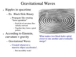
The L aser I nterferometer G ravitational-Wave O bservatory. The Search For Continuous Gravitational Waves. http://www.ligo.caltech.edu. Gregory Mendell, LIGO Hanford Observatory on behalf of the LIGO Science Collaboration. Supported by the United States National Science Foundation.

E N D
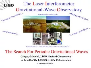
The Laser Interferometer Gravitational-Wave Observatory The Search For Continuous Gravitational Waves http://www.ligo.caltech.edu Gregory Mendell, LIGO Hanford Observatory on behalf of the LIGO Science Collaboration Supported by the United States National Science Foundation LIGO-G0900274-v2
Continuous Gravitational Waves The continuous gravitational wave signal from a triaxial rotating neutron star produces a strain h(t) with amplitude h0, and depends on the detector antenna patterns, F+ and F, inclination angle, , polarization angle , and phase . LIGO-G0900274-v2
-22 10 -23 10 Vela Crab -24 10 -25 strain PSR J1952+3252 (CTB80) 10 PSR J0537-6910 (LMC) J0437-4715 -26 10 -27 10 -28 10 0 1 2 3 10 10 10 10 GW frequency (Hz) Search sensitivity for a one year fully coherent search at LIGO’s S5 sensitivity For our fully coherent searches we use the maximum likelihood statistic, 2F, and a time-domain Bayesian approach. LIGO-G0900274-v2
Sensitivity: A Three Step Program With a signal, 2 PDF has noncentrality parameter d2 = optimal SNR2. 2F PDF is 2 for 4 degrees of freedom. Step 1. The False Alarm Rate gives a threshold on the statistic, 2F. For a 1% False Alarm Rate this threshold is 2F = 13.3. Step 2. The False Dismissal Rate gives the optimal SNR2, d2, needed. For a 10% False Dismissal Rate, d2 = 20.7. LIGO-G0900274-v2
The SNR depends on sky position and source orientation. Equation (84) of JKS [1] gives the optimal SNR2 as: (1) Define the orientation factor, K2, as: (2) LIGO-G0900274-v2
Mean(K2) = 4/25 = 0.16 95% K2 values > 0.042 Histogram 10000 random K2 values: Step 3. Substituting d2 = 20.7, mean(K2) = 0.16, and Tcoh = Tobs(the observation time) into Eq. (1) and solving for h0 gives the sensitivity for a fully coherent search for finding sources with average orientation for a 1% False Alarm Rate and 10% False Dismissal Rate: (3) LIGO-G0900274-v2
Caveats • To achieve 90% detection efficiency (a 10% false dismissal rate) we need an SNR that is detected 95% of the time over 95% of the orientations (.95*.95 ~ 0.90). Thus, it is more appropriate to use K2 = 0.042 when estimating the sensitivity [2]. However, for a single template search the threshold on 2F can be closer to ~ 4 (for ~50% false alarm rate). This lowers d2 by about a factor of 4, which keeps the sensitivity about equal to that in Eq. (3) for known pulsars. • However, to search for unknown sources we search over many templates, typically billions in each ~1 Hz band. A higher threshold is needed to keep the False Alarm Rate down. Coincidence steps are used to further reduce this rate. • For the Einstein@Home S4 all-sky search, a threshold of 2F = 28 was used, and coincidence in 12 of 17 stretches of data with Tcoh = 30 hr was required. The resulting sensitivity for a 10% false dismissal rate was [5]: (4) LIGO-G0900274-v2
To optimize sensitivity: • Reduce the noise, S, by improving the instrument. • Lower the threshold on 2F, while keeping the False Alarm Rate near zero. (We do this by using a parameter space metric to use fewer templates, and by using vetoes that e.g., require coincidence amongst IFOs, identify instrument lines, or ignore low doppler shift sky regions.) • Increase the coherent integration time Tcoh, e.g., using a resampling technique to speed up the calculation of 2F. • Due to computational cost a hierarchical approach is needed that incoherently combines coherent stretches of data. We use 2F for the coherent step and the Hough Transform for the incoherent step in the current S5 E@H. Fast semicoherent methods like PowerFlux are also used. • For N coherent segments combined incoherently, the sensitivity scales as: (5) Data analysis theory looks for ways to make the coefficient in front of the right side as small as possible. LIGO-G0900274-v2
References [1] P.Jaranowski, A.Królak, B.Schutz, “Data analysis of gravitational wave signals from spinning neutron stars. I. The signal and its detection”,Phys Rev D58, 063001, (1998). [2] J. Betzwieser, “Analysis of spatial mode sensitivity of a gravitational wave interferometer and a targeted search for gravitational radiation from the Crab pulsar”, Phd Thesis MIT, (2007). [3] LIGO Scientific Collaboration: B. Abbott, et al, “Beating the spin-down limit on gravitational wave emission from the Crab pulsar”, ApJ Lett 45, 683, (2008). [4] LIGO Scientific Collaboration: B. Abbott, et al, M. Kramer, A. G. Lyne, “Upper limits on gravitational wave emission from 78 radio pulsars”, Phys Rev D76, 042001, (2007). [5] LIGO Scientific Collaboration: B. Abbott, “The Einstein@Home search for periodic gravitational waves in LIGO S4 data”, Phys Rev D79, 022001, (2009). [6] LIGO Scientific Collaboration: B. Abbott, et al, “All-sky LIGO Search for Periodic Gravitational Waves in the Early Fifth-Science-Run Data”, Phys Rev Lett 102, 111102 (2009). LIGO-G0900274-v2
END LIGO-G0900274-v2
Beating the Crab Spindown Limit We have beaten the spindown limit for the Crab [3]. Upper limits from S5 are shown as exclusion regions in the I- plane. Dashed horizontal lines are theoretical bounds on I. Less than 6% of the total power from spindown is emitted as GWs; ULs are h095% = 3.4 10-25. and = 1.8 10-4 using I= 1038 kg.m2 and r = 2 kpc. LIGO-G0900274-v2
Known Pulsar S3/S4 Results Upper limits on gravitational wave emission from 78 radio pulsars were set using S3/S4 data [4]. The best h095% UL is 2.6 10-25; the best UL is less than 10-6. The plot shows upper limits against sensitivity estimated from Eq. (3). LIGO-G0900274-v2
Einstein@Home S4 Results Examples of the first published Einstein@Home search results for unknown sources, using S4 data. Shown are all candidates with at least 7 coincidences out of 17 30 hour segments, and that passed a veto on sky positions with little Doppler modulation [5]. The top plot includes hardware injected signals. The bottom plot removes bands around the hardware injections' frequencies. No candidates survived the detection criteria of 12 coincidences. The estimated sensitivity for 90% detection confidence is in Eq. (4). LIGO-G0900274-v2
PowerFlux Early S5 Results Computationally efficient semicoherent methods are also used to look for unknown sources. PowerFlux results from the early part of S5 are shown [6]. Upper limits (95% CL) on pulsar gravitational wave amplitude h0 for equatorial (red), intermediate (green), and polar (blue) declination bands for best-case (lower curves) and worst-case (upper curves) pulsar orientations. LIGO-G0900274-v2
Frequency Time Incoherent Power Averaging • Break up data into N segments; FFT each segment. • Track the frequency. • StackSlide: add the power weighted by the noise inverse. • Hough: add 1 or 0 if power is above/below a cutoff. • PowerFlux: add power using weights that maximize SNR LIGO-G0900274-v2