Download

1 / 90
900 likes | 906 Views
MATS-30004. Quantitative Methods Dr Huw Owens www.personalpages.manchester.ac.uk/staff/huw.owens. Resources – Reference Books. Anderson, Sweeney and Williams “An Introduction to Management Science, quantitative approaches to decision making” 7th edition

E N D
MATS-30004 Quantitative Methods Dr Huw Owens www.personalpages.manchester.ac.uk/staff/huw.owens
Resources – Reference Books • Anderson, Sweeney and Williams “An Introduction to Management Science, quantitative approaches to decision making” 7th edition • Hamdy A Taha, “Operations Research, An Introduction”, 5th edition • Burley TA and O’Sullivan G, “Operational Research” • Lapin L, “Quantitative Methods for business decisions with cases”, 5th edition • Swift L and Piff S (2005), Quantitative Methods for business, management and finance, second edition, Palgrave Macmillan, ISBN 1-4039-3528-9. • Slack N, Chambers S and Johnston R (2004), Operations Management, fourth edition, Prentice Hall, ISBN 0-273-67906-6
Models for Inventory Control • Objectives of these lectures: • After these lectures you should be able to: • Understand the costs incurred in keeping inventory. • Formulate and solve a basic EOQ model. • Adapt the model to allow for lead time and shortages • Use the variability coefficient to assess whether demand is constant • Know something about “ABC” classification
What is Inventory? - 1 • Most businesses need to store goods or materials ready to sell to the customer or for a subsequent part of the manufacturing process. These stocks are known as inventory. • Typical items carried in inventory can include: • raw materials • purchased parts • components • subassemblies • work-in-progess • finished goods and supplies • Why keep inventory? • To supply demand and not lose trade • BUT to store inventory incurs storage costs and ties up capital!
What is Inventory? - 2 • Main reason that organisations maintain stock levels is it is difficult to predict: • Sales levels • Production times • Demand • Usage needs • Inventory serves as a “buffer” against uncertain and fluctuating usage – It keeps a supply of items available for use by the organisation. • BUT Maintaining inventory incurs costs such as: • Ordering costs (setup cost – flat charge for delivery and admin) • Unit costs (charge per item) • Holding costs (insurance, interest lost on capital, cost of storage) • Shortage costs (cost of placing an order for immediate delivery, cost of lost trade, loss of goodwill)
How can we minimise inventory costs? • To minimise inventory costs a manager may ask two questions: • How much should be ordered when the inventory for the item is replenished? • When should the inventory for a given item be replenished?
Generalised Inventory Model • Ultimate questions: • How much to order? • When to order? • Order quantity should represent the optimum quantity that should be ordered every time an order is placed • When to order depends on: • periodic review at equal time intervals - the time for acquiring a new order usually coincides with the beginning of each time interval; • continuous review - a review point is usually specified by the inventory level at which a new order must be placed.
Total inventory cost Setup cost Holding cost Shortage cost Purchasing cost = + + + Generalised Inventory Model • The order quantity (how much) and reorder point (when) are normally determined by minimising the total inventory cost that can be expressed as a function of these two variables. The total inventory cost is generally composed of the following components: • Purchasing Cost (size of order – price break or quantity discount) • Setup Cost (order frequency) • Holding Cost
Quantitative Inventory Models • How can quantitative models assist in the decision making process: • Deterministic inventory models, where it is reasonable to assume that the rate of demand for the item is constant or nearly constant; • Probabilistic inventory models, where the demand for item fluctuates and can be described in probabilistic terms; • Just-In-Time (JIT), a philosophy of material management and control, of which the primary objective is to eliminate all sources of waste, including unnecessary inventory.
Types of EOQ Model • Deterministic Inventory Models • Single Item Static Economic Order Quantity (EOQ) • Single Item Static EOQ with price breaks • Single Item Static EOQ with planned shortages. • Economic production-quantity model.
Types of EOQ Model • Probabilistic • Single-period inventory model with probabilistic demand • An order-quantity, reorder-point inventory model with probabilistic demand • A periodic-review model with probabilistic demand
Basic EOQ Model • Simplest and least realistic but the basis of many other models. • Assumptions : Stock levels are gradually depleted at a constant rate. • This means that demand is constant and when stock runs out a fixed-size batch is ordered and arrives instantaneously!
Inventory level y Average inventory y/2 t0=y/D Time Figure 1 Basic EOQ Model • D = demand rate for an item (quantity/unit time) • y = the order quantity = maximum inventory level • K = the setup cost every time an order is placed • h = the holding cost per item per unit time • TC = the total cost per unit time Max. inventory level
Total inventory cost Setup cost Holding cost = + • The setup cost equals to the product of the number of orders per unit time and the setup cost per order. That is, • The holding cost can be calculated by multiplying the average inventory level to the holding cost per item per unit time. The average inventory level in the EOQ model is ½ y. Therefore, Setup Cost= Holding Cost=
How much to order? • Hence, Total Cost = • How much to order? • 1) Differentiate TC with respect to y • 2) Let the above equal zero • 3) Rearrange the equation for y*, the optimal order quantity:
The corresponding cycle time is • And the minimal total inventory cost is
When to Order • The concept of inventory position is defined as the amount of inventory on hand plus the amount of inventory on order. • The when to order decision is expressed in terms of a reorder point – the inventory position at which a new order should be placed. • In practice, an order takes time to be filled. • The lag time from the point an order is placed until delivery is called the lead time (denoted L)
Reorder points L L Figure 2 • Figure 2 illustrates the situation where reordering occurs L time units before delivery is expected. Inventory
In general, the reordering point (R) can be calculated by the following equation: • R = L x D (3) • Where D is the demand per unit time and L is the lead time. • NOTE: The lead time L may either be longer or shorter than the cycle time t0. • If L<t0, use L directly in equation 3. • If L>t0, (L-nt0) should be used in equation 3 instead of L where n is the largest integer not exceeding
An Example • The daily demand for a commodity is approximately 100 units. Every time an order is placed, a fixed cost K of £100 is incurred. The daily holding cost h per unit is 2 pence. If the lead time is 12 days determine the economic order quantity and the reorder point. • We know • K=£100 per order • D= 100 units per day • h=£0.02 per unit per day • L=12 days • Using equation 1, • And the cycle time is • Because in this case L>t0, the reorder point is calculated as
Try for yourself • R=(L-t0) x D = (12-10) x 100 = 200 units • Therefore, it is most economical to order 1000 units of the commodity when the inventory level reaches 200 units. • One for you to try: • A video manufacturer produces 8000 video recorders on a continuous production line every month. Each video recorder requires a tape head unit and these are produced very quickly in batches. It costs £12,000 to set up the machinery to produce a batch and 30p a month to store and insure a tape head unit once made. How large should the batch size be to minimise total costs and how often will they need to set up a production run?
Try for yourself • We know • K=£12,000 per order • D= 8000 units per day • h=£0.30 per unit per day • As only 8000 units are required each month, 25,298 units will last 25,298/8000 = 3.16225 months. So the manufacturer should produce a batch of tape head units every 3.16 months.
Questions • Suppose the demand for a product occurs evenly at a rate of 20 units per week. Every time an order is placed a cost of £15 is incurred and it costs £0.2 per item a week to insure the goods and £0.1 per item per week to store the goods. How frequently should an order be placed and how many units should be ordered in a batch? • Matthews Motor Homes sell, on average, 5 Harvey models a week. The local supplier charges a flat rate of £1000 for each delivery regardless of size. Garaging costs for each motor home work out at £20 per week and insurance is £25 per motor home per week. Matthews prefer to place a regular, fixed-size order with the supplier and shortages are not allowed. How many Harveys should Matthews order in a batch, and how often? What assumptions are implicit here?
Answers • 1) D=20, K=15 and h=0.2+0.1=0.3. So • EOQ = sqrt((2*20*15)/0.3) = 44.72 • And the cycle length will be 44.72/20 = 2.24 weeks. So an order of 45 units should be placed every 2.25 weeks. • 2) D=5, K=1000, h=45. So • EOQ=sqrt((2*1000*5)/45) = 14.9 • And the cycle length should be 14.9/5 = 3 weeks. The model assumes that delivery is immediate and that demand occurs at a constant rate.
Lecture 2 Single Item Static (EOQ) with price breaks • In the basic EOQ model purchasing cost per unit time is assumed to be constant and should not affect the level of inventory. • BUT, usually there are price breaks or quantity discounts and these should be included in the model. • For example, consider the inventory model with instantaneous stock replenishment and no shortages. • We’ll assume cost per unit is • C1 for y < q and • C2 for y q • Where C1 > C2 and q is the quantity above which a price break is guaranteed • The TC per unit time will now include the purchasing cost in addition to the setup cost and the holding cost
Cost TC1 TC2 I II III ym q1 y Figure 3 • The total cost per unit time with price break is 4 These two functions are shown graphically in Figure 3. Disregarding the effect of price breaks for the moment, we let ym be the quantity at which the minimum values of TC1 and TC2 occur.
Thus, • The cost functions TC1 and TC2 in Figure 4 reveal that the determination of the optimum order quantity y* depends on where q, the price break point falls with respect to the three zones I, II and III as shown in Figure 3. • These zones are defined by determining q1 (>ym) from the equation • TC1(ym)=TC2(q1) • Since ym is known, the solution will yield the value q1.
Cost Cost Cost TC1 TC1 TC2 TC2 I I I II II II III III III ym ym ym q1 q1 q1 y y y • The optimum order quantity y* is illustrated in Figure 4 TC2 TC1 q q q Figure 4
Determining y* • Determine If q < ym (zone I), then y*=ym, and the procedure ends. Otherwise, • Determine q1 from equation TC1 (ym)=TC2(q1) and decide whether q falls in zone II or zone III. • If ym < q < q1 (zone II), then y* = q; • If q>=q1 (zone III), then y*=ym.
Example • Consider the inventory model with the following information. K = £10, h = £1, D = 5 units, c1 = £2, c2 =£1, and q = 15 units. • First, we need to compute the ym. • ym = (2KD/h) = (2105/1) = 10 units • Since q > ym, it is necessary to check whether q is in zone II or zone III. The value of q1 is computed from • TC1 (ym) = TC2 (q1) • namely, DC1 + KD/ym + ½ hym = DC2 + KD/q1 + ½ hq1 • Substitution yields • q12 - 30q1 + 100 = 0 • This is obviously of the type ax2 + bx + c = 0 whose solutions are • So, the solutions for q1 are found to be either q1 = 26.18 units or q1 = 3.82 units. By definition, q1 must be larger than ym. Therefore, q1 = 26.18 units. Since ym < q < q1, q is in zone II. Therefore, the optimum order quantity y* = q = 15 units. • The associated total cost per unit time is • TC2(y*) = TC2 (15) = DC2 + KD/15 + 15h/2 = £15.83/day.
EOQ model with planned shortages • A shortage is a demand that cannot be supplied. • Shortages are usually undesirable and should be avoided. • BUT for situations with high commodity unit cost values (e.g. cars) shortages are desirable and often used. • In this model, the assumptions are: • the shortage cost is small; • no demand is lost because of shortage as the customers will back order, i.e., accept delayed delivery (this type of shortage being known as backorders); and • the replenishment is instantaneous.
y t2 t1 b T Figure 5 EOQ model with planned shortages • y = the total ordering quantity • D = Demand rate of the commodity • b = the inventory shortage, or the backorder • t1 = the time units in which the inventory reaches the zero level • t1 = (y-b)/D • t2 = the time period from stock-out to the arrival of a new order • t2 = b/D • T = the inventory cycle, T = y/D • p = shortage penalty
In this case, the total inventory cost can be expresses as the sum of the holding cost, setup cost, and the shortage cost: • TC = holding cost + setup cost + shortage cost • Holding Cost • The holding cost per cycle consists of 2 parts. The first part of the cycle lasts whilst the maximum stock level is used up; that is for (y-b) time units. During this time the average stock level is (y-b)/2, so the holding cost per cycle is
Shortage Cost • Shortage Cost • If we assume that the shortage penalty is p per item per unit time, then the shortage cost is • p average backorder level • Since the average backorder level is • the shortage cost is • b2p/(2y ) (cost /unit time) • Therefore, the total cost is • (cost/unit time) (5)
Shortage Cost • Minimise TC with respect to the order quantity and to the planned backorders yields the optimal values of order quantity y* and backorder b*: • (6) (7) • Proof • That gives
Shortage Cost • Substituting in the above equation gives • From equation (6), The interval between orders can be calculates as follows: • (8)
Setup cost • It is known from the EOQ model that the cost per order is K. The setup cost equals to K multiplying the number of orders in the given period of time. • The number of orders can be calculated by dividing the demand by the ordering quantity, i.e., D/y. The setup cost rate is K per order, hence the total setup cost is • KD/y (cost/unit time)
An Example - 1 • Suppose the North-west Electronics Company has a product for which the assumptions of the EOQ inventory model with backorders are valid. Information obtained by the company is as follows: • The annual demand D = 2000 units/year • The cost per order K = £25 • The holding cost rate h = £10 per unit per year • The backorder cost p = £30 per unit per year • Work out the optimal order quantity y*, the optimal backorder level b*, and the cycle time T. • Solve: • The optimal order quantity • y* = [2200025/10 (10+30)/30] = 115.47 units 115 units • The optimal backorder level • b* = 10/(10+30) 115 = 28.75 units 29 units
An Example - 2 • The cycle time for place orders • T = y*/D = 115/2000 = 0.0575 year • Since there are 250 working days in a year, the cycle time is 0.0575250 = 14.4 working days. • The total annual cost for operating the inventory is • TC = holding cost • + setup cost • + shortage cost • = (10(115-29)2)/(2115) • + (200025)/115 • + (29230)/(2115)
= £322 + £435 + £110 = £867/year • If the company had chosen to prohibit backorders and had adopted the regular EOQ model, the recommended inventory decision would have been • y* = (2200025/10) = 100 units
Questions • Suppose the North-west Electronics Company has a product for which the assumptions of the EOQ inventory model with backorders are valid. Information obtained by the company is as follows: • The annual demand D = 1000 units/year • The cost per order K = £15 • The holding cost rate h = £12 per unit per year • The backorder cost p = £20 per unit per year • Work out the optimal order quantity y*, the optimal backorder level b*, and the cycle time T.
Economic production-quantity model • In previous models we have assumed that orders will be delivered instantaneously but this is not very realistic! • Consider the following situation, • When the inventory reaches its zero level, a production system starts its operation and adds new items to the inventory while the inventory keeps on its normal operation. (Of course, the production rate of items must be higher than that of the demand rate.)
Production rate y Demand rate Max inv. level T2 T1 T Figure 6 Economic production-quantity model • D = the demand rate per unit time • P = the production rate per unit time • h = the holding cost per item per unit time • K = the setup cost every time an order is placed
Economic production-quantity model • As in the EOQ model, we are now dealing with two costs, the holding cost and the setup cost. Namely • TC = holding cost + setup cost • Holding cost • We know that the holding cost is equal to the product of the average inventory level and the holding cost per item per unit time. Let • D = the demand rate per unit time • P = the production rate per unit time • h = the holding cost per item per unit time • Then, as in Figure 6, T = y/D, T1 = y/P, and T2 = T - T1 = y(P-D) / DP
Economic production-quantity model • The maximum inventory level in this situation is • the build-up speed T1 = (P-D) y/P = y(P-D)/P • From the EOQ model, we know that the average inventory level is half of its maximum. In this case, it is ½ y(P-D)/P. Therefore, • the holding cost = ½ y(P-D)/P h = ½ yh(P-D)/P • Setup cost • The setup cost is based on the number of production runs per unit time and the setup cost per run. • The number of production runs is D/y. If the setup cost per run is K, which includes the labour, material, and other relevant cost during the production, then the setup cost is • the setup cost = D/y K = DK/y
Economic production-quantity model • Total cost • The total cost for this model is • TC = ½ yh(P-D)/P + DK/y (9) • The minimum-cost production quantity, often referred to as the economic production quantity, can be found by minimise TC with respect to y, leading to • (10)
EPQ Model Example 1 • Example • Beauty Bar Soap is produced on a production line that has an annual capacity of 60,000 cases. The annual demand is estimated 26,000 cases, with the demand rate essentially constant throughout the year. The cleaning, preparation, and setup of the production line cost approximately $135. The manufacturing cost per case is $4.50, and the annual holding cost is figured at a 24% rate. Thus the holding cost per case per year is h = 0.24 $4.50 = $1.08. What is the recommended production quantity? • Solve: • We know that • P = 60,000 cases/year • D = 26,000 cases/year • K = $135 per run • h = $1.08 per case per year
EPQ Model Example 1 • So, • cases • The total annual cost according to y* is • TC* = = $2073 • The cycle time between production runs is • T = y*/D = 3387/26000 = 0.1327 year • Considering that there are 250 working days in a year, • T = 250 0.1327 33 working days • Thus, we should plan a production run of 3387 units about every 33 working days.
Probabilistic Models • In reality many inventory situations cannot be described by deterministic models. • In these cases, the demand is no longer constant and deterministic but probabilistic. • We can describe this type of demand using a probability distribution.
Probability 1 • Is it likely to rain tomorrow? • How can we measure probability? • When outcomes are equally likely (e.g. a coin toss) • When outcomes are not equally likely (e.g. getting run over by a car!) • Subjective probability (‘Gut Feeling’) • Outcome – the result of a chance situation such that a list of all possible outcome covers every possibility (it is exhaustive) and no outcome overlaps any of the others (we say the outcomes are mutually exclusive)