Adjoint modeling and applications

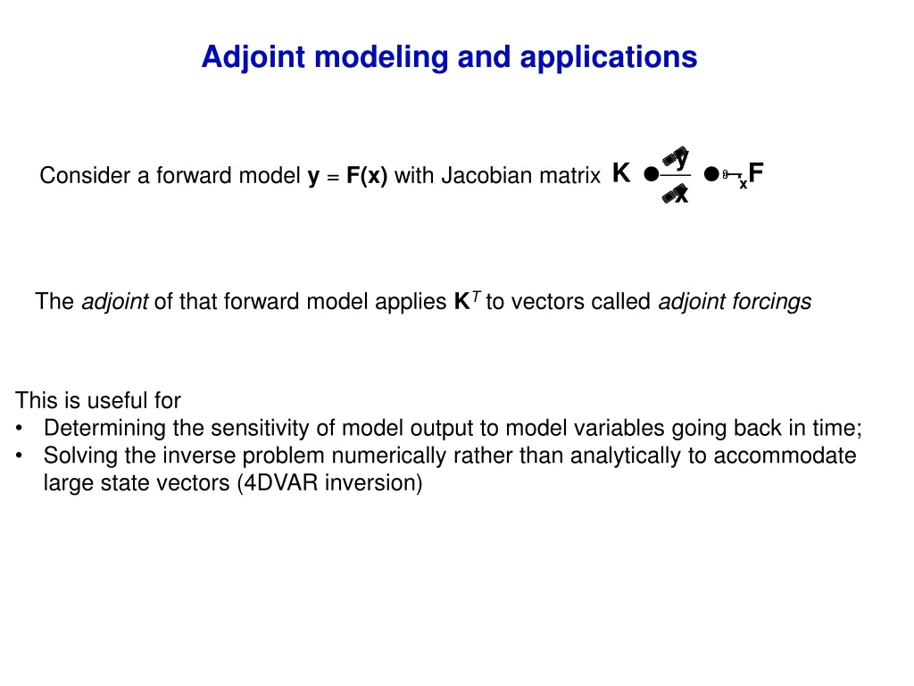
1. Adjoint modeling and applications Consider a forward model y = F(x) with Jacobian matrix The adjoint of that forward model applies KT to vectors called adjoint forcings • This is useful for • Determining the sensitivity of model output to model variables going back in time; • Solving the inverse problem numerically rather than analytically to accommodate large state vectors (4DVAR inversion)

2. Forward model (CTM): Adjoint model as sensitivity analysis tool State vector x(0) Concentrations y(0)y(1) y(p-1)y(p) Time t0 t1 tp-1 tp Jacobian expresses sensitivity of y(p) to x(0): Take transpose: Apply sequentially to unit vector v = (1,0…0)T: followed by etc… Single pass of the adjoint over [tp, t0] returns sensitivity of y(p),1to all model variables at all previous times: y(p),1/y(p-1), y(p),1/y(p-2),… y(p),1/x(0)

3. Application to receptor modeling: sensitivity of smoke in Singapore to fire locations in Equatorial Asia MODIS fire observations, June 20-29 2013 Smoke in Singapore, June 20 Smoke transport simulated by GEOS-Chem • Large fire emissions in Equatorial Asia from oil palm and timber plantations • Adjoint can identify the sensitivity of smoke concentrations at a particular receptor site to fire emissions at all locations and previous times Smoke concentration in surface air Kim et al. [2015]

4. Using GEOS-Chem adjoint to compute sensitivity of smoke concentrations in Singapore to fire emissions Emissions E(x, t) from bottom-up inventory Concentrations y(x, t) =F(E(x, t)) computed with GEOS-Chem Sensitivities s (x, t,t’) = ySingapore(t)/E(x, t’) computed with GEOS-Chem adjoint Contributions to Singapore smoke Smoke concentrations in Singapore can be calculated for ANY emission inventory Eand time t using archived sensitivities computed just ONCE from the adjoint:

5. Consider a CTM split into advection (A), chemistry (C), and emission (E) operators: Linearize each operator so that it operates as a matrix: Simple construction of a CTM adjoint This defines the Tangent Linear Model (TLM) and the model adjoint: TLM Adjoint Constructing the adjoint requires construction of the TLM by differentiating the model equations or the model code…and this represents most of the work

6. transpose (adjoint) α α α 1 2 3 Courant number α = ut/ x Adjoint of a linear advection operator Linear upstream advection scheme: Transpose applies reverse winds: Same applies in a linear Lagrangian model (reverse the winds to get the adjoint)

7. Adjoint of a linear chemistry operator A linear chemistry operator is self-adjoint; same operator can be used in forward and adjoint models. Sensitivity with respect to emissions is also self-adjoint:

8. Variational inversion A Solve the inverse problem xA ° 1 2 ° x1 numerically rather than analytically ° x2 1. Starting from prior xA, calculate 2. Using a steepest-descent algorithm get next guess x1 3. Calculate 3 x3 ° , get next guess x2 4. Iterate until convergence Adjoint model computes by applying KT to adjoint forcings Minimum of cost function J

9. Adjoint method for calculating cost function gradient Time t0 t1 tp-2 tp-1 tp Observations y(0)y(1)y(p-2)y(p-1)y(p) Forward model F(xA) over[t0, tp] add add add add t0 t1 tp-2 tp-1 tp adjoint model

10. State vector: 3-D time-dependent concentration field (very large) Observation vector: observations of state variables or related variables 3DVAR and 4DVAR data assimilation Example: assimilation of satellite observations of stratospheric ozone 3DVAR 3DVAR 3DVAR 4DVAR 4DVAR t0 t1 = t0 + h t2 = t0 + 2h Forecast model with assimilation at time increments h 3DVAR: same as Kalman filter but minimize cost function numerically 4DVAR: use adjoint to optimize field at t0 using observations spread over [t0, t0 + h]