Download
1 / 18
180 likes | 315 Views
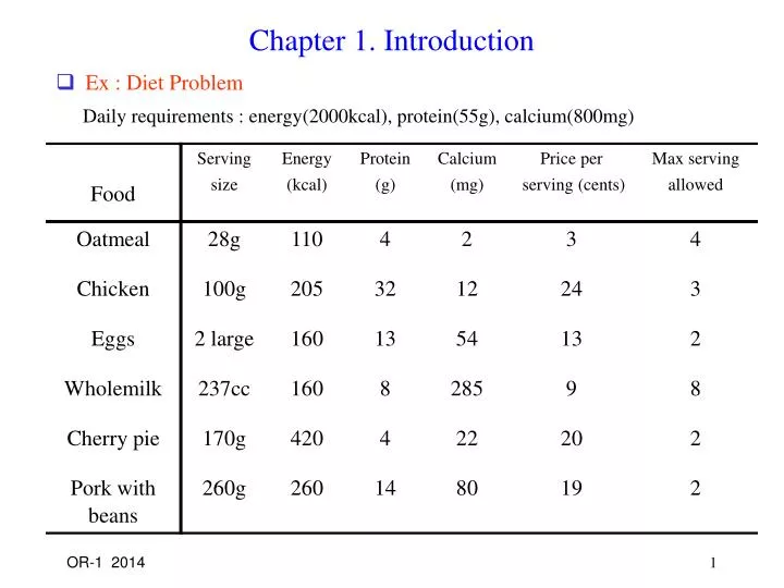
Chapter 1. Introduction. Ex : Diet Problem Daily requirements : energy(2000kcal), protein(55g), calcium(800mg). Formulation:. Subject to. Linear Programming Problem ( 선형계획법 문제 ). objective function ( 목적함수 ). right hand side ( 우변상수 ). Constraints ( 제약식 ). Subject to.

E N D
Chapter 1. Introduction • Ex : Diet Problem Daily requirements : energy(2000kcal), protein(55g), calcium(800mg)
Formulation: Subject to
Linear Programming Problem (선형계획법 문제) objective function (목적함수) right hand side (우변상수) Constraints (제약식) Subject to nonnegativity constraints (비음제약식) (may not exist for some variables, then they are called unrestricted or freevariables)
Unusual formulations • Cutting stock problem : (Refer Chapter 13) Rolls of papers (called raws) with width to be cut into small pieces(finals). pieces of width , need to be produced. How to cut the rolls to meet demands while minimizing wastes? minimize s. t. , and integer for all • Consider possible cutting patterns for a raw. : number of rolls to be cut using -th cutting pattern. denotes the total number of possible patterns which can be a very large number. if the number of finals produced in the j-th pattern is .
ex) raws W=100 in., need 97 finals of width 45 in. 610 finals of width 36 in. 395 finals of width 31 in. 211 finals of width 14 in. Min x1 + x2 + x3 + … + x37 • Note: • number of patterns grows fast as problem becomes large (We don’t solve the problem with all columns in the model. We start with a few columns and solve the LP, and then identify and add a new column to the model and solve the LP again, … (column generation method). • round down fractional optimal solution to LP to obtain integer solution, then use a few more raws to meet demands. • extensions to 2-dimensional cutting stock (nesting problem), 3-D packing
Piecewise linear convex function: Consider , (maximum of affine functions, called a piecewise linear convex function.)
Thm: Let be convex functions. Then is also convex. pf) =
, . min s. t. , s.t., , • Minimization of piecewise linear convex function
ex)parallel processor scheduling problem There are processors and jobs to be processed on any one of the processors. : processing time of job on processor . Assign jobs to processors so that overall finish time (makespan) is minimized. Formulation as an integer programming problem. Let = 1 if job is assigned to processor , 0 otherwise. minimize {} s. t. , and integer for all minimize s. t. , , and integer for all
Linear programming relaxation of an integer programming problem is obtained by dropping the integrality requirements on the variables and considering only the linear constraints. • The optimal value of the linear programming relaxation provides a lower bound (for the minimization problem) on the optimal value of the integer programming problem. Hence it can be used importantly in the algorithm for integer programming problem. ( Integer Program: min , , and integer. Let , be the optimal value of the integer program (IP) and its LP relaxation, respectively. Let be the optimal solution of IP, then is a feasible solution to LP relaxation. Hence .) • For the maximization problem, LP relaxation gives an upper bound on the optimal value of IP. • Note that maximize cannot be formulated as a linear programming problem. (maximizing a convex function)
Special case of piecewise linear objective function : separable piecewise linear objective function. • function is called separable if . If objective function is nonlinear, but separable we may approximate it by piecewise linear function. (need some caution) • The cost structure may be progressive, e.g.: electricity cost. slope: 0
Ex: Suppose = 1, = 2, = 3, = 4 = 5, = 10, = 15 If = 7, we want to have = + + + = 5 + 2 + 0 + 0 and objective function value is = 15 + 22 + 30 + 4 0 = 9 • Replace in the constraints with , where 0 , 0 , 0 , 0 In the objective function, use : min Since we solve minimization problem, it is guaranteed that if we get in an optimal solution , have values at their upper bounds. • Ex(continued): = 7 may be expressed 5 + 0 + 2 + 0 with = 5, = 0, = 2, = 0. But then, objective function value is = 15 + 20 + 32 + 4 0 = 11, which is worse than the previous solution. (We have a minimization problem.)
Terminology • Feasible solution (가능해) : vector that satisfies all constraints • Optimal solution (최적해) : feasible solution that gives the largest objective function value. • Optimal value (최적값) : objective function value of an optimal solution. • Infeasible LP : LP that does not have a feasible solution • Unbounded : LP is called unbounded if there exists a feasible solution that gives optimal value > for any finite > 0. ex: {max , s.t.} • Every LP has one of the following three statuses: • There exists an optimal solution with finite optimal value (There may exist multiple optimal solutions) • Infeasible • Unbounded
Brief History of LP • Solving systems of linear inequalities : Fourier, 1826, not efficient (Chapter 16) • Simplex method : G. B. Dantzig, 1947 • Ellipsoid method : L. G. Khachian, 1979 First polynomial time algorithm (theoretically efficient algorithm) for LP, practically not good. • Interior point method : L. Karmarkar, 1984 polynomial time algorithm, many variations, practically good performance. Recently, used for some nonlinear programming problems successfully (convex program – min convex function, convex set) • Theory of LP provides important foundation for many other disciplines like integer programming, networks and graphs, nonlinear programming, etc .
Standard form • (In vector notation) maximize maximize s. t. , s.t. , • Any LP problem can be expressed as the standard form • Minimization problem : solve max , then take the negative of the optimal objective value. Optimal solution is the same • Equality constraint : , • Unrestricted variable substitute by (in the objective function and in the constraints where . (Simplex method finds an optimal solution with at most one of is positive) • Some people use min(max) as standard form.
ex) max max s. t. s. t.
Formulation when absolute values appear in the objective function (Assume cj 0 for variables involving absolute values) min min s. t. , s.t., unrestricted for all for all • Express free variable as () in the constraints () Also in the objective function as ()(). We want = , if = , if We need in an optimal solution, i.e. at most one of is positive. If for all , this is guaranteed to hold at an optimal solution.
Ex: Suppose = 3, = 5 = 0 – 5 in an optimal solution, hence objective value is 3 (0 + 5) = 15. If we have = 2, = 7, then = 2 7 = – 5. But objective value is 3 (2 + 7) = 27, which is inferior compared to the previous solution. Hence at most one of is positive at an optimal solution. • Alternative formulation: minimize s. t. , , ,