Download
1 / 88
880 likes | 949 Views
Recognition of regulatory signals. Mikhail S. Gelfand IntegratedGenomics-Moscow NATO ASI School, October 2001. Why?. Additional annotation tool (e.g. specificity of transporters and enzymes from large families) Important for practice (in addition to metabolic reconstruction)

E N D
Recognition of regulatory signals Mikhail S. Gelfand IntegratedGenomics-Moscow NATO ASI School, October 2001
Why? • Additional annotation tool (e.g. specificity of transporters and enzymes from large families) • Important for practice (in addition to metabolic reconstruction) • Interesting from the evolutionary point of view
Overview 0. Biological introduction 1. Algorithms • Representation of signals • Deriving the signal • Site recognition 2. Comparative genomics • Phylogenetic footprinting • Consistency filtering
Some biology • Transcription (DNA RNA) • Splicing (pre-mRNA mRNA) • Translation (mRNA protein) • Regulation of transcription in prokaryotes • … and eukaryotes • Initiation of translation
Representation of signals • Consensus • Pattern (consensus with degenerate positions) • Positional weight matrix (PWM, or profile) • Logical rules • RNA signals
Consensus codB CCCACGAAAACGATTGCTTTTT purE GCCACGCAACCGTTTTCCTTGC pyrD GTTCGGAAAACGTTTGCGTTTT purT CACACGCAAACGTTTTCGTTTA cvpA CCTACGCAAACGTTTTCTTTTT purC GATACGCAAACGTGTGCGTCTG purM GTCTCGCAAACGTTTGCTTTCC purH GTTGCGCAAACGTTTTCGTTAC purL TCTACGCAAACGGTTTCGTCGG consensus ACGCAAACGTTTTCGT
Pattern codB CCCACGAAAACGATTGCTTTTT purE GCCACGCAACCGTTTTCCTTGC pyrD GTTCGGAAAACGTTTGCGTTTT purT CACACGCAAACGTTTTCGTTTA cvpA CCTACGCAAACGTTTTCTTTTT purC GATACGCAAACGTGTGCGTCTG purM GTCTCGCAAACGTTTGCTTTCC purH GTTGCGCAAACGTTTTCGTTAC purL TCTACGCAAACGGTTTCGTCGG consensus ACGCAAACGTTTTCGT pattern aCGmAAACGtTTkCkT
Frequency matrix Information content I = j bf(b,j)[log f(b,j) / p(b)]
Probabilistic motivation: log-likelihood (up to a linear transformation) • More probabilistic motivation: z-score (with the suitable base of the logarithm) • Thermodynamical motivation: free energy (assuming independence of positions, up to a linear transformation) • Pseudocounts
Compilation of samples • Initial sample: • GenBank • specialized databases • literature (reviews) • literature (original papers) • Correction of GenBank errors • Checking the literature • removal of predicted sites • Removal of duplicates
Re-alignment approaches • Initial alignment by a biological landmark • start of transcription for promoters • start codon for ribosome binding sites • exon-intron boundary for splicing sites • Deriving the signal within a sliding window • Re-alignment • etc. etc. until convergence
Gene starts of Bacillus subtilis dnaN ACATTATCCGTTAGGAGGATAAAAATG gyrA GTGATACTTCAGGGAGGTTTTTTAATG serS TCAATAAAAAAAGGAGTGTTTCGCATG bofA CAAGCGAAGGAGATGAGAAGATTCATG csfB GCTAACTGTACGGAGGTGGAGAAGATG xpaC ATAGACACAGGAGTCGATTATCTCATG metS ACATTCTGATTAGGAGGTTTCAAGATG gcaD AAAAGGGATATTGGAGGCCAATAAATG spoVC TATGTGACTAAGGGAGGATTCGCCATG ftsH GCTTACTGTGGGAGGAGGTAAGGAATG pabB AAAGAAAATAGAGGAATGATACAAATG rplJ CAAGAATCTACAGGAGGTGTAACCATG tufA AAAGCTCTTAAGGAGGATTTTAGAATG rpsJ TGTAGGCGAAAAGGAGGGAAAATAATG rpoA CGTTTTGAAGGAGGGTTTTAAGTAATG rplM AGATCATTTAGGAGGGGAAATTCAATG
dnaN ACATTATCCGTTAGGAGGATAAAAATG gyrA GTGATACTTCAGGGAGGTTTTTTAATG serS TCAATAAAAAAAGGAGTGTTTCGCATG bofA CAAGCGAAGGAGATGAGAAGATTCATG csfB GCTAACTGTACGGAGGTGGAGAAGATG xpaC ATAGACACAGGAGTCGATTATCTCATG metS ACATTCTGATTAGGAGGTTTCAAGATG gcaD AAAAGGGATATTGGAGGCCAATAAATG spoVC TATGTGACTAAGGGAGGATTCGCCATG ftsH GCTTACTGTGGGAGGAGGTAAGGAATG pabB AAAGAAAATAGAGGAATGATACAAATG rplJ CAAGAATCTACAGGAGGTGTAACCATG tufA AAAGCTCTTAAGGAGGATTTTAGAATG rpsJ TGTAGGCGAAAAGGAGGGAAAATAATG rpoA CGTTTTGAAGGAGGGTTTTAAGTAATG rplM AGATCATTTAGGAGGGGAAATTCAATG cons. aaagtatataagggagggttaataATG num. 001000000000110110000000111 760666658967228106888659666
dnaN ACATTATCCGTTAGGAGGATAAAAATG gyrA GTGATACTTCAGGGAGGTTTTTTAATG serS TCAATAAAAAAAGGAGTGTTTCGCATG bofA CAAGCGAAGGAGATGAGAAGATTCATG csfB GCTAACTGTACGGAGGTGGAGAAGATG xpaC ATAGACACAGGAGTCGATTATCTCATG metS ACATTCTGATTAGGAGGTTTCAAGATG gcaD AAAAGGGATATTGGAGGCCAATAAATG spoVC TATGTGACTAAGGGAGGATTCGCCATG ftsH GCTTACTGTGGGAGGAGGTAAGGAATG pabB AAAGAAAATAGAGGAATGATACAAATG rplJ CAAGAATCTACAGGAGGTGTAACCATG tufA AAAGCTCTTAAGGAGGATTTTAGAATG rpsJ TGTAGGCGAAAAGGAGGGAAAATAATG rpoA CGTTTTGAAGGAGGGTTTTAAGTAATG rplM AGATCATTTAGGAGGGGAAATTCAATG cons. tacataaaggaggtttaaaaat num. 0000000111111000000001 5755779156663678679890
Positional information content before and after re-alignment
Positional nucleotide frequencies after re-alignment (aGGAGG pattern)
Deriving the signal ab initio • “Discrete” (pattern-driven) approaches: word counting • “Continuous” (profile-driven) approaches: optimization
Word counting. Short words • Consider all k-mers • For each k-mer compute the number of sequences containing this k-mer • (maybe with some mismatches) • Select the most frequent k-mer
Problem:Complete search is possible only for short words Assumption: if a long word is over-represented, its subwords also are overrepresented Solution: select a set of over-represented words and combine them into longer words
Word counting. Long words • Consider somek-mers • For each k-mer compute the number of sequences containing this k-mer • (maybe with some mismatches) • Select the most frequent k-mer
Problem:what k-tuples to start with? 1st attempt: those actually occurring in the sample. But: the correct signal (the consensus word) may not be among them.
2nd attempt: those actually occurring in the sample and some neighborhood. But: • again, the correct signal (the consensus word) may not be among them; • the size of the neighborhood grows exponentially
Graph approach Each k-mer in each sequence corresponds to a vertex. Two k-mers are linked by an arc, if they differ in at most h positions (h<<k). Thus we obtain an n-partite graph (n is the number of sequences). A signal corresponds to a clique (a complete subgraph) – or at least a dense subgraph – with vertices in each part.
A simple algorithm • Remove vertices that cannot be extended to complete subgraphs • that is, do not have arcs to all parts of the graph • Remove pairs that cannot be extended … • that is, do not form triangles with the third vertex in all parts of the graph • Etc. (will not work “as is” for dense subgraphs)
Optimization. EM algorithms • Generate an initial set of profiles (e.g. seed with all k-mers) • For each profile • find the best (highest scoring) representative in each sequence • update the profile • Iterate until convergence
This algorithm converges. However, it cannot leave the basin of attraction. Thus, if the initial approximation is bad, it will converge to nonsense. Solution: stochastic optimization.
Simulated annealing • Goal: maximize the information content I I = j bf(b,j)[log f(b,j) / p(b)] • or any other measure of homogeneity of the sites
Let A be the current signal (set of candidate sites), and let I(A) be the corresponding information content. Let B be a set of sites obtained by randomly choosing a different site in one sequence, and let I(B)be its information content. • if I(B) I(A), B is accepted • if I(B) < I(A), B is accepted with probability P =exp [(I(B) – I(A)) / T] The temperature T decreases exponentially, but slowly; the initial temperature is chosen such that almost all changes are accepted.
Gibbs sampler Again, A is a signal (set of sites), and I(A) is its information content. At each step a new site is selected in one sequence with probability P ~exp [(I(Anew)] For each candidate site the total time of occupation is computed. (Note that the signal changes all the time)
Use of symmetry • DNA-binding factors and their signals • Co-operative homogeneous • Palindromes • Repeats • Co-operative non-homogeneous • Cassetes • Others • RNA signals
Recognition: PWM/profiles The simplest technique: positional nucleotide weights are W(b,j)=ln(N(b,j)+0.5) – 0.25iln(N(i,j)+0.5) Score of a candidate site b1…bk is the sum of the corresponding positional nucleotide weights: S(b1…bk ) = j=1,…,kW(bj,j)
Distribution of RBS profile scores on sites (green) and non-sites (red)
Pattern recognition • Linear discriminant analysis • Logical rules • Syntactic analysis • Context-sensitive grammars • Perceptron • Neural networks
Neural networks: architecture • 4kinput neurons (sensors), each responsible for observing a particular nucleotide at particular position OR 2k neurons (one discriminates between purines and pyrimidines, the other, between AT and GC) • One or more layers of hidden neurons • One output neuron
Each neuron is connected to all neurons of the next layer • Each connection is ascribed a numerical weight A neuron • Sums the signals at incoming connections • Compares the total with the threshold (or transforms it according to a fixed function) • If the threshold is passed, excites the outcoming connections (resp. sends the modified value)
Training: • Sites and non-sites from the training sample are presented one by one. • The output neuron produces the prediction. • The connection weights and thresholds are modified if the prediction is incorrect. Networks differ by architecture, particulars of the signal processing, the training schedule