Download
1 / 64
650 likes | 666 Views
Digital Image Processing. Spatial Filtering. Christophoros Nikou cnikou@cs.uoi.gr. Contents. In this lecture we will look at spatial filtering techniques: Neighbourhood operations What is spatial filtering? Smoothing operations What happens at the edges? Correlation and convolution

E N D
Digital Image Processing Spatial Filtering ChristophorosNikou cnikou@cs.uoi.gr
Contents In this lecture we will look at spatial filtering techniques: • Neighbourhood operations • What is spatial filtering? • Smoothing operations • What happens at the edges? • Correlation and convolution • Sharpening filters • Combining filtering techniques
Neighbourhood Operations Origin x (x, y) Neighbourhood y Image f (x, y) Neighbourhood operations simply operate on a larger neighbourhood of pixels than point operations Neighbourhoods are mostly a rectangle around a central pixel Any size rectangle and any shape filter are possible
Simple Neighbourhood Operations Some simple neighbourhood operations include: • Min: Set the pixel value to the minimum in the neighbourhood • Max: Set the pixel value to the maximum in the neighbourhood • Median: The median value of a set of numbers is the midpoint value in that set (e.g. from the set [1, 7, 15, 18, 24] 15 is the median). Sometimes the median works better than the average
Simple Neighbourhood Operations Example Original Image Enhanced Image x x 123 127 128 119 115 130 140 145 148 153 167 172 133 154 183 192 194 191 194 199 207 210 198 195 164 170 175 162 173 151 y y
The Spatial Filtering Process a b c d e f g h i r s t u v w x y z Origin x * Original Image Pixels Filter Simple 3*3Neighbourhood 3*3 Filter e eprocessed = v*e + r*a + s*b + t*c + u*d + w*f + x*g + y*h + z*i y Image f (x, y) The above is repeated for every pixel in the original image to generate the filtered image
Spatial Filtering: Equation Form Images taken from Gonzalez & Woods, Digital Image Processing (2002) Filtering can be given in equation form as shown above Notations are based on the image shown to the left
Smoothing Spatial Filters One of the simplest spatial filtering operations we can perform is a smoothing operation • Simply average all of the pixels in a neighbourhood around a central value • Especially useful in removing noise from images • Also useful for highlighting gross detail Simple averaging filter
Smoothing Spatial Filtering 104 100 108 99 106 98 95 90 85 1/9 1/9 1/9 1/9 1/9 1/9 1/9 1/9 1/9 104 100 108 1/9 1/9 1/9 1/9 1/9 1/9 99 98 95 90 85 1/9 1/9 1/9 Origin x * Original Image Pixels Filter Simple 3*3Neighbourhood 3*3 SmoothingFilter 106 e = 1/9*106 + 1/9*104 + 1/9*100 + 1/9*108 + 1/9*99 + 1/9*98 + 1/9*95 + 1/9*90 + 1/9*85 = 98.3333 y Image f (x, y) The above is repeated for every pixel in the original image to generate the smoothed image.
Image Smoothing Example Images taken from Gonzalez & Woods, Digital Image Processing (2002) The image at the top left is an original image of size 500*500 pixels The subsequent images show the image after filtering with an averaging filter of increasing sizes • 3, 5, 9, 15 and 35 Notice how detail begins to disappear
Weighted Smoothing Filters More effective smoothing filters can be generated by allowing different pixels in the neighbourhood different weights in the averaging function • Pixels closer to the central pixel are more important • Often referred to as a weighted averaging Weighted averaging filter
Another Smoothing Example Original Image Smoothed Image Thresholded Image Images taken from Gonzalez & Woods, Digital Image Processing (2002) By smoothing the original image we get rid of lots of the finer detail which leaves only the gross features for thresholding
Averaging Filter Vs. Median Filter Example Original ImageWith Noise Image AfterAveraging Filter Image AfterMedian Filter Images taken from Gonzalez & Woods, Digital Image Processing (2002) Filtering is often used to remove noise from images Sometimes a median filter works better than an averaging filter
Spatial smoothing and image approximation Images taken from Gonzalez & Woods, Digital Image Processing (2002) Spatial smoothing may be viewed as a process for estimating the value of a pixel from its neighbours. What is the value that “best” approximates the intensity of a given pixel given the intensities of its neighbours? We have to define “best” by establishing a criterion.
Spatial smoothing and image approximation (cont...) Images taken from Gonzalez & Woods, Digital Image Processing (2002) A standard criterion is the the sum of squares differences. The average value
Spatial smoothing and image approximation (cont...) Images taken from Gonzalez & Woods, Digital Image Processing (2002) Another criterion is the the sum of absolute differences. There must be equal in quantity positive and negative values.
Spatial smoothing and image approximation (cont...) Images taken from Gonzalez & Woods, Digital Image Processing (2002) • The median filter is non linear: • It works well for impulse noise (e.g. salt and pepper). • It requires sorting of the image values. • It preserves the edges better than an average filter in the case of impulse noise. • It is robust to impulse noise at 50%.
Spatial smoothing and image approximation (cont...) Images taken from Gonzalez & Woods, Digital Image Processing (2002) Example edge Impulse noise Median (N=3) Average (N=3) The edge is smoothed
Strange Things Happen At The Edges! e e e e e e At the edges of an image we are missing pixels to form a neighbourhood Origin x e y Image f (x, y)
Strange Things Happen At The Edges! (cont…) There are a few approaches to dealing with missing edge pixels: • Omit missing pixels • Only works with some filters • Can add extra code and slow down processing • Pad the image • Typically with either all white or all black pixels • Replicate border pixels • Truncate the image • Allow pixels wrap around the image • Can cause some strange image artefacts
Strange Things Happen At The Edges! (cont…) Filtered Image: Zero Padding Filtered Image: Replicate Edge Pixels OriginalImage Images taken from Gonzalez & Woods, Digital Image Processing (2002) Filtered Image: Wrap Around Edge Pixels
Correlation & Convolution a b c d e e f g h r s t u v w x y z Original Image Pixels Filter The filtering we have been talking about so far is referred to as correlation with the filter itself referred to as the correlation kernel Convolution is a similar operation, with just one subtle difference For symmetric filters it makes no difference. eprocessed = v*e + z*a + y*b + x*c + w*d + u*e + t*f + s*g + r*h *
Effect of Low Pass Filtering on White Noise Let fbe an observed instance of the image f0 corrupted by noise w: with noise samples having mean value E[w(n)]=0 and being uncorrelated with respect to location:
Effect of Low Pass Filtering on White Noise (cont...) Applying a low pass filter h(e.g. an average filter)by convolution to the degraded image: The expected value of the output is: The noise is removed in average.
Effect of Low Pass Filtering on White Noise (cont...) What happens to the standard deviation of g? Let where the bar represents filtered versions of the signals, then
Effect of Low Pass Filtering on White Noise (cont...) Considering that h is an average filter, we have at pixel n: Therefore,
Effect of Low Pass Filtering on White Noise (cont...) Sum of squares Cross products
Effect of Low Pass Filtering on White Noise (cont...) Sum of squares Cross products (uncorrelated as ml)
Effect of Low Pass Filtering on White Noise (cont...) Finally, substituting the partial results: The effect of the noise is reduced. This processing is not optimal as it also smoothes image edges.
Sharpening Spatial Filters Previously we have looked at smoothing filters which remove fine detail Sharpening spatial filters seek to highlight fine detail • Remove blurring from images • Highlight edges Sharpening filters are based on spatial differentiation
Spatial Differentiation Images taken from Gonzalez & Woods, Digital Image Processing (2002) Differentiation measures the rate of change of a function Let’s consider a simple 1 dimensional example
Spatial Differentiation Images taken from Gonzalez & Woods, Digital Image Processing (2002) A B
Derivative Filters Requirements First derivative filter output • Zero at constant intensities • Non zero at the onset of a step or ramp • Non zero along ramps • Second derivative filter output • Zero at constant intensities • Non zero at the onset and end of a step or ramp • Zero along ramps of constant slope
1st Derivative The formula for the 1st derivative of a function is as follows: It’s just the difference between subsequent values and measures the rate of change of the function
1st Derivative (cont.) • The gradient of an image: The gradient points in the direction of most rapid increase in intensity. Gradient direction The edge strength is given by the gradient magnitude Source: Steve Seitz
2nd Derivative The formula for the 2nd derivative of a function is as follows: Simply takes into account the values both before and after the current value
Using Second Derivatives For Image Enhancement Edges in images are often ramp-like transitions • 1st derivative is constant and produces thick edges • 2nd derivative zero crosses the edge (double response at the onset and end with opposite signs) A common sharpening filter is the Laplacian • Isotropic • One of the simplest sharpening filters • We will look at a digital implementation
The Laplacian The Laplacian is defined as follows: where the partial 1st order derivative in the x direction is defined as follows: and in the y direction as follows:
The Laplacian (cont…) 0 1 0 1 -4 1 0 1 0 So, the Laplacian can be given as follows: We can easily build a filter based on this
The Laplacian (cont…) Images taken from Gonzalez & Woods, Digital Image Processing (2002) OriginalImage LaplacianFiltered Image LaplacianFiltered ImageScaled for Display Applying the Laplacian to an image we get a new image that highlights edges and other discontinuities
But That Is Not Very Enhanced! LaplacianFiltered ImageScaled for Display Images taken from Gonzalez & Woods, Digital Image Processing (2002) The result of a Laplacian filtering is not an enhanced image We have to do more work in order to get our final image Subtract the Laplacian result from the original image to generate our final sharpened enhanced image
Laplacian Image Enhancement Images taken from Gonzalez & Woods, Digital Image Processing (2002) In the final sharpened image edges and fine detail are much more obvious - = OriginalImage LaplacianFiltered Image SharpenedImage
Laplacian Image Enhancement Images taken from Gonzalez & Woods, Digital Image Processing (2002)
Simplified Image Enhancement The entire enhancement can be combined into a single filtering operation
Simplified Image Enhancement (cont…) 0 -1 0 -1 5 -1 0 -1 0 Images taken from Gonzalez & Woods, Digital Image Processing (2002) This gives us a new filter which does the whole job for us in one step
Simplified Image Enhancement (cont…) Images taken from Gonzalez & Woods, Digital Image Processing (2002)
Variants On The Simple Laplacian 0 -1 1 1 -1 1 0 -1 1 1 -1 1 -8 -4 9 1 1 -1 1 0 -1 1 1 -1 1 0 -1 Images taken from Gonzalez & Woods, Digital Image Processing (2002) There are lots of slightly different versions of the Laplacian that can be used: SimpleLaplacian Variant ofLaplacian