Download
1 / 18
200 likes | 452 Views
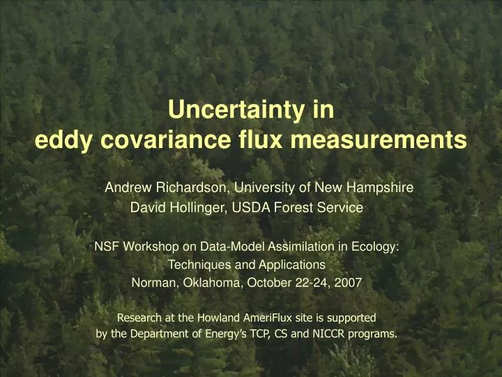
Uncertainty in eddy covariance flux measurements. Andrew Richardson, University of New Hampshire David Hollinger, USDA Forest Service NSF Workshop on Data-Model Assimilation in Ecology: Techniques and Applications Norman, Oklahoma, October 22-24, 2007

E N D
Uncertainty in eddy covariance flux measurements Andrew Richardson, University of New Hampshire David Hollinger, USDA Forest Service NSF Workshop on Data-Model Assimilation in Ecology: Techniques and Applications Norman, Oklahoma, October 22-24, 2007 Research at the Howland AmeriFlux site is supported by the Department of Energy’s TCP, CS and NICCR programs.
"To put the point provocatively, providing data and allowing another researcher to provide the uncertainty is indistinguishable from allowing the second researcher to make up the data in the first place." Raupach et al. (2005). Model data synthesis in terrestrial carbon observation: methods, data requirements and data uncertainty specifications. Global Change Biology 11:378-97.
Measurement uncertainty and parameter uncertainty • The observed data are just one realization, drawn from a “statistical universe of data sets” (Press et al. 1992) • Different realizations of the random draw lead to different estimates of “true” model parameters • Parameters estimates are therefore themselves uncertain (but we want to describe their distributions!) A statistical universe
What uncertainty? • A measurement is never perfect - data are not “truth” (corrupted truth?) • “Uncertainty” describes the inevitable error of a measurement: x´ = x + + • x´ is what is actually measured; it includes both systematic () and random () components • typically, is assumed Gaussian, and is characterized by its standard deviation, ()
examples: nocturnal biases imperfect spectral response advection energy balance closure operate at varying time scales: fully systematic vs. selectively systematic variety of influences: fixed offset vs. relative offset cannot be identified through statistical analyses can correct for systematic errors (but corrections themselves are uncertain) uncorrected systematic errors will bias DMF analyses examples: surface heterogeneity and time varying footprint turbulence sampling errors measurement equipment (IRGA and sonic anemometer) random errors are stochastic; characteristics of pdf can be estimated via statistical analyses (but may be time-varying) affect all measurements cannot correct for random errors random errors limit agreement between measurements and models, but should not bias results Random errors Systematic errors
Uncertainty at various time scales • Monte Carlo simulations suggest that uncertainty in annual NEE integrals uncertainty is ± 30 g C m-2 y-1 at 95% confidence (combination of random measurement error and associated uncertainty in gap filling) • Systematic errors accumulate linearly over time (constant relative error) • Random errors accumulate in quadrature (so relative uncertainty decreases as flux measurements are aggregated over longer time periods)
Random flux uncertainties are non-Gaussian with non-constant variance • Simultaneous measurements at 2 towers (Howland) • Hollinger & Richardson (2005) Tree Physiology. • Single tower, next day comparisons (Howland, Harvard, Duke, Lethbridge, WLEF, Nebraska) • Richardson et al. (2006) Agric. & For. Meteorol. • Data-model residuals • Hagen et al. (2006) JGR • Richardson & Hollinger (2005) Agric. & For. Meteorol. • Richardson et al. (2007) Agric. & For. Meteorol. These characteristics violate two key assumptions of least-squares fitting!
A method to estimate the distribution of Repeated measurements: Use simultaneous, but independent, measurements from two towers, x´1and x´2 Howland: Main and West towers • same environmental conditions • similar patches of forest • non-overlapping footprints (independent turbulence) Then: If x´ = x + and cov(x´1, x´2)=0 (x´1 – x´2) = x´1) + x´2) – 2cov(x´1, x´2) () = (x´1 – x´2)/2 x´1 ~800m x´2
A double exponential (Laplace) pdf better characterizes the uncertainty • Strong central peak & • heavy tails (leptokurtic) • non-Gaussian pdf Better: double-exponential pdf, f(x) = exp(|x/|)/2 The double-exponential is characterized by the parameterb
The standard deviation of the uncertaintyscales with the magnitude of the flux • Larger fluxes are more uncertain than small fluxes • Relative error decreases with flux magnitude • Large errors are not uncommon • 95% CI = ± 60% • 75% CI = ± 30% To obtain maximum likelihood parameter estimates, cannot use OLS: must account for the fact that the flux measurement errors are non-Gaussian and have non-constant variance.
Generality of results • Scaling of uncertainty with flux magnitude has been validated using data from a range of forested CarboEurope sites: y-axis intercept (base uncertainty) varies among sites (factors: tower height, canopy roughness, average wind speed), but slope constant across sites (Richardson et al., 2007) • Similar results (non-Gaussian, heteroscedastic) have been demonstrated for measurements of water and energy fluxes (H and LE) (Richardson et al., 2006) • Results are in agreement with predictions of Mann and Lenschow (1994) error model based on turbulence statistics (Hollinger & Richardson, 2005; Richardson et al., 2006)
Maximum likelihood paradigm: “what model parameters values are most likely to have generated the observed data, given the model and what is known about measurement errors?” Assumptions about errors affect specification of the ML cost function: Other cost functions are possible! For Gaussian data (“weighted least squares”) For double exponential data (“weighted absolute deviations”)
Specifying a different cost function affects optimal parameter estimates • Lloyd & Taylor (1994) respiration model: Reco –respiration T –soil temperature A, E0, T0 – parameters • model parameters differ depending on how the uncertainty is treated (explanation: nocturnal errors have slightly skewed distribution) • Why? error assumptions influence form of likelihood function
Influence of cost function specification on model predictions • Half-hourly model predictions depend on parameter-ization; integrated annual sum decreases by ~10% decrease (≈40% of NEE) when absolute deviations is used • Influences NEE partitioning, annual sum of GPP • Trivial model but relevant example
Summary • Knowledge of measurement uncertainty is critical for inverse modeling and advanced analysis techniques • Random flux measurement error is reasonably well described by a double exponential pdf (it is not Gaussian!) • Flux measurement error is heteroscedastic – uncertainty scales with magnitude of flux (it is not constant!)
Conclusion • “Data uncertainties are as important as the data themselves” (Raupach et al. 2005) because specification of uncertainties affects the uncertainty of the model as well as the model predictions themselves. • Should use weighted absolute deviations rather than ordinary least squares when specifying the cost function for most DMF exercises involving eddy flux data (aside: implications of CLT for aggregated data).