Download
1 / 30
320 likes | 1.12k Views
Testing Assumptions of Linear Regression. Detecting Outliers Transforming Variables Logic for testing assumptions. Assumptions of regression.

E N D
Testing Assumptions of Linear Regression • Detecting Outliers • Transforming Variables • Logic for testing assumptions
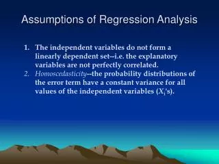
Assumptions of regression • Based on information from the data set 2001WorldFactbook.sav, is the following statement true, false, or an incorrect application of a statistic? Assume that the assumptions of linear regression are satisfied. Use .05 for alpha in the regression analysis and .01 for the diagnostic tests. • A simple linear regression between "population growth rate" [pgrowth] and "birth rate" [birthrat] will satisfy the regression assumptions if we choose to interpret which of the following models. • 1 The original variables including all cases • 2 The original variables excluding extreme outliers • 3 The transformed variables including all cases • 4 The transformed variables excluding extreme outliers *** • 5 The quadratic model including all cases • 6 The quadratic model excluding extreme outliers • 7 None of the proposed models satisfies the assumptions • The transformed variables excluding extreme outliers is the correct answer. [Feedback: 4743 characters] • TESTING MODEL: ORIGINAL VARIABLES, USING ALL CASES • The linear regression of "birth rate" [birthrat] by "population growth rate" [pgrowth] satisfied one of the regression assumptions (independence of errors). The Durbin-Watson statistic (1.93) fell within the acceptable range from 1.50 to 2.50, indicating that the assumption of independence of errors was satisfied. • However, three assumptions were violated (linearity, homogeneity of error variance, and normality of the residuals). The lack of fit test (F(157, 59) = 1.78, p = .006) indicated that the assumption of linearity was violated. The Breusch-Pagan test (Breusch-Pagan(1) = 679.27, p < .001) indicated that the assumption of homogeneity of error variance was violated. The Shapiro-Wilk test of studentized residuals (Shapiro-Wilk(218) = 0.81, p < .001) indicated that the assumption of normality of errors was violated. • TESTING MODEL: ORIGINAL VARIABLES, OMITTING EXTREME OUTLIERS • One extreme outliers were found in the data. Montserrat was an extreme outlier (the cook's distance (21.295252) was larger than the cutoff value of 0.037037,the leverage (0.331496) was larger than the cutoff value of 0.036697 and the studentized residual (-9.173) was smaller than the cutoff value of -4.0). • The linear regression of birthrat by "population growth rate" [pgrowth] satisfied two of the regression assumptions (linearity and independence of errors). The lack of fit test (F(156, 59) = 0.94, p = .617) indicated that the assumption of linearity was satisfied. The Durbin-Watson statistic (2.01) fell within the acceptable range from 1.50 to 2.50, indicating that the assumption of independence of errors was satisfied. • However, two assumptions were violated (homogeneity of error variance and normality of the residuals). The Breusch-Pagan test (Breusch-Pagan(1) = 29.24, p < .001) indicated that the assumption of homogeneity of error variance was violated. The Shapiro-Wilk test of studentized residuals (Shapiro-Wilk(217) = 0.97, p < .001) indicated that the assumption of normality of errors was violated. • SELECTING A TRANSFORMATION • The logarithm of "birth rate" [LG_birthrat] with a value of 0.957 for the Shapiro-Wilk statistic was the transformation that was most normal for the dependent variable "birth rate" [birthrat]. • The logarithm of "population growth rate" [LG_pgrowth] with a value of 0.975 for the Shapiro-Wilk statistic was the transformation that best approximated a normal distribution for the independent variable "population growth rate" [pgrowth]. • TESTING MODEL: TRANSFORMED VARIABLES, INCLUDING ALL CASES • The linear regression of logarithm of "birth rate" [LG_birthrat] by logarithm of "population growth rate" [LG_pgrowth] satisfied two of the regression assumptions (linearity and independence of errors). The lack of fit test (F(157, 59) = 1.38, p = .080) indicated that the assumption of linearity was satisfied. The Durbin-Watson statistic (1.94) fell within the acceptable range from 1.50 to 2.50, indicating that the assumption of independence of errors was satisfied. • However, two assumptions were violated (homogeneity of error variance and normality of the residuals). The Breusch-Pagan test (Breusch-Pagan(1) = 29.02, p < .001) indicated that the assumption of homogeneity of error variance was violated. The Shapiro-Wilk test of studentized residuals (Shapiro-Wilk(218) = 0.96, p < .001) indicated that the assumption of normality of errors was violated. • TESTING MODEL: TRANSFORMED VARIABLES, EXCLUDING EXTREME OUTLIERS • One extreme outliers were found in the data. Montserrat was an extreme outlier (the cook's distance (21.295252) was larger than the cutoff value of 0.037037,the leverage (0.331496) was larger than the cutoff value of 0.036697 and the studentized residual (-9.173) was smaller than the cutoff value of -4.0). • The linear regression of logarithm of "birth rate" [LG_birthrat] by logarithm of "population growth rate" [LG_pgrowth] satisfied all of the regression assumptions (linearity, homogeneity of error variance, normality of the residuals, and independence of errors). • The lack of fit test (F(156, 59) = 1.14, p = .288) indicated that the assumption of linearity was satisfied. The Breusch-Pagan test (Breusch-Pagan(1) = 0.82, p = .367) indicated that the assumption of homogeneity of error variance was satisfied. The Shapiro-Wilk test of studentized residuals (Shapiro-Wilk(217) = 0.99, p = .357) indicated that the assumption of normality of errors was satisfied. The Durbin-Watson statistic (1.96) fell within the acceptable range from 1.50 to 2.50, indicating that the assumption of independence of errors was satisfied.
Run the script - 1 Select Run Script from the Utilities menu.
Run the script - 2 Navigate to the folder where you downloaded the script. Highlight the script (.SBS) file to run. Click on the Run button to run the script.
Assumption of linearity - 1 Click on the arrow button to move the variable to the text box for the dependent variable. Highlight the dependent variable in the list of variables.
Assumption of linearity - 1 Highlight the independent variable in the list of variables. Click on the arrow button to move the variable to the list box for the independent variable.
Initial test of conformity to assumptions Run the regression with all cases to test the initial conformity to the assumptions.
The Durbin-Watson statistic (1.93) fell within the acceptable range from 1.50 to 2.50, indicating that the assumption of independence of errors was satisfied.
The lack of fit test (F(157, 59) = 1.78, p = .006) indicated that the assumption of linearity was violated.
The Breusch-Pagan test (Breusch-Pagan(1) = 679.27, p < .001) indicated that the assumption of homogeneity of error variance was violated.
The Shapiro-Wilk test of studentized residuals (Shapiro-Wilk(218) = 0.81, p < .001) indicated that the assumption of normality of errors was violated.
One extreme outliers were found in the data. Montserrat was an extreme outlier (the cook's distance (21.295252) was larger than the cutoff value of 0.037037,the leverage (0.331496) was larger than the cutoff value of 0.036697 and the studentized residual (-9.173) was smaller than the cutoff value of -4.0).
We could exclude the cases one at a time by selecting the case in the list of cases included and clicking on the arrow button, or we can use the script. The script will remove the extreme outliers by clicking on the Exclude extreme outliers button.
Case number 136, Montserrat, is added to the list of cases to exclude.
To see whether or not removing the outlier resolves the violation of assumptions, run the regression again. Run the regression with all cases to test the initial conformity to the assumptions.
This is an example of a strong linear relationship. The red lowess (loess in SPSS) smoother is almost completely straight throughout the range of the data. The rate of change in the dependent variable is the same for all values of the independent variable.
Removing the one extreme outlier solved the violation of the assumption of linearity. The lack of fit test (F(156, 59) = 0.94, p = .617) indicated that the assumption of linearity was satisfied.
The Durbin-Watson statistic (2.01) fell within the acceptable range from 1.50 to 2.50, indicating that the assumption of independence of errors was satisfied.
The Breusch-Pagan test (Breusch-Pagan(1) = 29.24, p < .001) indicated that the assumption of homogeneity of error variance was violated.
The Shapiro-Wilk test of studentized residuals (Shapiro-Wilk(217) = 0.97, p < .001) indicated that the assumption of normality of errors was violated.
Since removing outliers did not solve all of our violations, we will try transformations of the variables. We restore all of the cases to the analysis by clicking on the Include all cases button.
First, click on the dependent variable to select it. Click on the Test normality button.
There is a statistical procedure named the Box-Cox transformation which SPSS does not compute and which I have not added to the script. However, we can use the test of normality as a surrogate. As the statistical value of the Shapiro-Wilk statistic gets larger, it is associated with a higher probability. We will select the transformation with the largest Shapiro-Wilk statistic as the transformation which best “normalizes” the variable, provided it is at least 0.01 larger than the statistical value for the untransformed variable. For this variable, we would choose the Logarithmic transformation. Choosing one transformation does not mean that is is particularly effective, only that it is better than the others.
First, click on the dependent variable to select it. Click on the Test normality button.
First, click on the dependent variable to select it. Click on the Test normality button.
First, click on the dependent variable to select it. Click on the Test normality button.
First, click on the dependent variable to select it. Click on the Test normality button.
First, click on the dependent variable to select it. Click on the Test normality button.
First, click on the dependent variable to select it. Click on the Test normality button.
Since removing outliers did not solve all of our violations, we will try transformations of the variables. We restore all of the cases to the analysis by clicking on the Include all cases button.