Download
1 / 57
620 likes | 678 Views
Introduction to ellipsometry J.Ph.PIEL (PhD) Application Lab Manager SOPRALAB. OUTLINE : Basic Theory GES5 description Data Analysis Conclusion. I - BASIC THEORY Brief history of Ellipsometry Principle Physical meaning of y and D.

E N D
Introduction to ellipsometry J.Ph.PIEL (PhD) Application Lab Manager SOPRALAB
OUTLINE : • Basic Theory • GES5 description • Data Analysis • Conclusion
I - BASIC THEORY • Brief history of Ellipsometry • Principle • Physical meaning of y and D
For the 1st time Paul DRUDE use ellipsometry in 1888 Phase measurement 2000
AlexandreRothen Published in 1945 a paper where the word « Ellipsometer » appears for the 1st time Thickness sensitivity : 0.3 A
Bref Historique Schematic representation of the mounting from Alexandre Rothen (Rev. of scientifique instruments Feb 1945)
Few key people in ellipsometry area • Malus in 1808 :discovery of the polarisation of light by reflexion. • Fresnel in 1823 : Wave theory of the light. • Maxwell in 1873 : developpment of the Electrogmagnetic field theory. • Drude in 1888 : Use of the extreme sensitivity of the ellipsometry to detect ultra thin layers (monolayer). • Abeles in 1947 : Developpment of matrix formalism applied to thin layers stack. • Rothe in 1945 : Introduction of the word : « Ellipsometer » • Hauge, Azzam, Bashara in 1970 : description and developpement of different ellipsometer settings. • 1980 : development of « Personal Computer » , automatisation of the technique. Industrial development of tools.
INTRODUCTION ELLIPSOMETRY is a method based on measurement of the change of the polarisation state of light after reflection at non normal incidence on the surface to study -The measurement gives two independent angles: and - It is an absolute measurement: do not need any reference - It is a non-direct technique: does not give directly the physical parameters of the sample (thickness and index) - It is necessary to always use a model to describe the sample SPECTROSCOPIC ELLIPSOMETRY (SE) gives more comprehensive results since it studies material on a wide spectral range
elliptical polarisation linear polarisation q0 Ep.rp Es. rs Ep Es Er Ei Ambient (n0, k0) EP Ei rp Er rs ES Thin Film 1 (n1, k1, T1) Thin Film 2 (n2, k2, T2) Thin Film i (ni, ki, Ti) Substrate (ns, ks) rp rs = tan Ψ.e jD= f( ni, ki, Ti ) r = PRINCIPLE OF SPECTROSCOPIC ELLIPSOMETRY Ellipsometry measures the complex reflectance ratio :
- After reflection on the sample, the extremity of the electric field vector describes an ellipse p e rp Y rs 0 s - This ellipse is characterised by *the ellipticity Tan e which is the ratio of the large axis to the small axis *the angle of rotation between the main axis and the P axis:
Physical meaning of y and D. • Those parameters give all relevant information about the polarization state of the light at a given wavelength. • - Tan y gives exactly the angle of the first diagonal ofthe rectangle in which the ellipse is enclosed. • - Cos D gives roughly how fat is going to be the ellipse (shape). • Its mathematically linked to the ratio of short axis to long axis of the ellipse in its fundamental frame. However, y and D are not straightforwardly linked to the easiest geometrical features of the ellipse. q :angle of rotation of the long axis of the ellipse versus axis p
Example of some different phase shift (D) for a given y value. • On those graphics, the long axis is the ellipse is represented and it has to be compared with the diagonal of the rectangle. • Because y is fixed, the ellipse is enclosed in the same rectangle for each graphic. • Modification of D change both angle of inclination and ellipticity.
II - GES5 DESCRIPTION • Physical description • Jones Formalism • Mathematical treatment of the signal • Example
Microspots Goniometer Polariser Arm Analyser Arm Mapping rho/theta Sample
SPECTROSCOPIC ELLIPSOMETER Goniometer Xe Lamp A P Optical Fiber Photo Multiplier Tube Scanninig channel C.C.D. channel
Schematics of dispersion elements Spectrograph Entrance Fiber Multichannel Detector Grating : fixed Spectrometer Entrance Fiber Grating : rotating PMT Prism : rotating NIR detector
GENERAL GES5 DESCRIPTION: • - Xenon Lamp:75 W, Short arc, High brilliance • - MgF2 Rotating Polarizer MgF2 : 6 Hz • - Adjustable Analyzer • Goniometer from 7° up to 90° • Microspots : spot size : 400 µm • High resolution way : • Spectral range : 190 nm up to 2000 nm- resolution < 0.5 nm • double monochromator: prism + grating • Photon counting PMT • High speed way : • Spectral range : 190 nm up to 1700 nm • Measurement duration : few seconds • Fixed grating spectrograph • CCD (1024x64 pixels)and OMA NIR (256 pixels) detectors
Jones Formalism BUT : Jones formalism can only work if there is no depolarisation effects induced by the material
Optical system with no depolarisation effects is characterized by this following Jones Matrix : 2X2 complex Matrix
If the material is isotrope : Ellipsometric Angles Y and D measured simultaneously
Px = Pq = Jones Matrix for a Linear Polarizer : Rotation Matix : General expression for a polarizer where the main axis is oriented with an angle q Pq =R(-q).Px.R(q)
I = Edp . Edp* + Eds . Eds* I (t) = I0 . ( 1 + a Cos 2 (t) + b Sin 2 (t) ) A : Angle between Analyser and plane of Incidence. (t) : Angle between Polariseur and plane of Incidence.
Edp 1 0 Cos A Sin A rp 0 Cos P - Sin P 1 0 Ep Eds 0 0 -Sin A Cos A 0 rs Sin P Cos P 0 0 Es = Detector Analyser Rotation Sample Rotation Polariser Lamp I = Edp . Edp* + Eds . Eds* I = I0 . ( 1 + a Cos 2 P(t) + b Sin 2 P(t) ) A : Angle between Analyser axis and Plane of Incidence. P(t) : Angle between Polarizer axis and Plane of Incidence.
[S1 + S2 + S3 + S4 ] P [S1 + S2 - S3 - S4 ] 2 I0 [S1 - S2 -S3 + S4 ] 2 I0 I0 = b = a = HADAMART TRANSFORM Intensity S1 S2 S3 S4 S1 Time
Cos 2 A Tan 2Y + Tan 2 A I0 = Tan 2Y - Tan 2 A Tan 2Y + Tan 2 A 2 Cos D . Tan Y. Tan A Tan 2Y + Tan 2 A a = b = 1 + a 1 - a Tan Y = Tan A . b 1 - a2 Cos D = CALCULATION OF THE ELLIPSOMETRIC PARAMETERS
DUV UV VISIBLE NIR ELLIPSOMETRIC MEASUREMENT
Physical Model Estimated sample structure TanY Experimental Measurement - Film Stack and structure - Material n, k, dispersion - Composition Fraction of Mixture CosD No Yes Experimental Measurement = Model Simulation ? Ti , ni , ki RESULTS ANALYSIS • Non direct technique. • Need the use of models to interpret the measurements and to get physical parameters of the layers REAL SAMPLE STRUCTURE
III - DATA ANALYSIS • Which physical parameters can we get ? • Sensisitivy of the technique • Description of the main models used • How to describe optical properties of the materials.
Which physical parameters can we get ? • Mechanical thickness of each layer : • Monolayer sensitivity (<0.01 A) up to 50 µm. • Refractive index versus wavelength : n(l) • Allow to characterize the quality of the layer and the process. • Extinction coefficient versus wavelength: k(l). • Measure the attenuation of light in the material. • Allow to characterize the quality of the layer and the process. • Surface and Interface characterization. • Layer inhomogeneity characterization. • In case of metallic or activated doping material: • resistivity and doping concentration characterization using Drude Model. • In case of porous material: porosity, pore size distribution and Young modulus characterization using Kelvin model.
Angle of incidence: 75° Spectroscopic ellipsometry sensitiviy Phase variation : is extremelly sensitive to ultra thin layers
Angle of incidence: 75° Spectroscopic ellipsometry sensitiviy Sensitivity could reach 0.01 A or 1 picometer 0nm 10 A
2 media model : Substrat alone Fresnel equation and Snell-Descartes law: rp = (ns.cosf0 – n0.cosfs)/(ns.cosf0+ ns.cosf1) and rs= (n0.cosf0 - ns.cosfs)/(ns.cosf0 + ns.cosf1) with r = rp/ rs = TanY.exp(i.D) F0 Ambiant : air Substrat ns = ñs - i.ks F1 Direct inversion of the ellipsometric parameters to get substrate indices ns = sinf0.(1 + ((1-r)/(1+r))2.Tan2f0)1/2
2 media model : Substrat alone Angle of incidence 75° Silicium
SiO2 30.8 Å Sicr 3 media model : one layer on known substrate Native oxide (SiO2) on Silicon
SiO2 1200 Å Sicr 3 media model : one layer on known substrate SiO2 layer on silicon
SiO2 1,9838µm Sicr 3 media model : one layer on known substrate Thick SiO2 layer on Silicon
3 media model : one layer on known substrate Rp et Rs are periodic function Same periods Idem for Tan Y and Cos D If fa =75° Period=l/(nb2-0.93)0.5 For SiO2 film nb =1.5 Period = l/2.3 At l=450 nm, period = 200 nm Sensitivity to D : In this case D variation de 360° for a period = 200 nm D sensitivity given by instrument: 5.10-2° Thickness sensitivity : 0.01 A
Multilayer stack Propagation inside the layer : Interferences Interface relations : Fresnel -
How to describe optical properties of the materials • Index library • Effective medium mixing laws • Dispersion law • Harmonic oscillators laws • Drude laws
Index Library • 3 main type of materials: • Dielectric : transparent in the visible range but absorbing in the UV and have absorbing band in the IR. • Transparent materials : Oxides (SiO2, TiO2) Fluorides (MgF2) • Optical filters, Anti reflective coatings, dielectric mirror (lasers). • Semi-conductors dispersives laws extremelly rich in the visible range linked to the band structures. Could be metallic in the IR. • Silicon : Si; Germanium : Ge; Gallium arsenide : GaAs; • Gallium nitride: GaN; • Carbon Silicon SiC (blue diode); • Metal highly absorbing in the visible. • Infrared mirrors :Au, Al, Cu • Magnetic Materials : Co, Ni, Fe, Gd • Handbook of Optical Constants from Palick • SOPRA library • Direct measurements on bulk materials
Interface and Surface roughnesstreated by Effective medium Model
Limits of the effective medium model • Model is convenient for physical or mechanical mixing. • Ex : Porous material with inclusion of void. • Model is not convenient for chemical mixing • Ex : Inclusion of atom in elementary cells • or variable atomic concentration • Ex : Si(1-x)Gex. • - Model is not applicable when the size of inhomogeneities • exceed few hundredth (1/100) of the wavelenght of the beam.