Download
1 / 31
310 likes | 400 Views
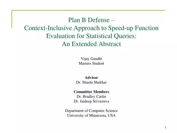
Plan B Defense – Context-Inclusive Approach to Speed-up Function Evaluation for Statistical Queries: An Extended Abstract. Vijay Gandhi Masters Student Advisor Dr. Shashi Shekhar Committee Members Dr. Bradley Carlin Dr. Jaideep Srivastava Department of Computer Science

E N D
Plan B Defense –Context-Inclusive Approach to Speed-up Function Evaluation for Statistical Queries: An Extended Abstract Vijay Gandhi Masters Student Advisor Dr. Shashi Shekhar Committee Members Dr. Bradley Carlin Dr. Jaideep Srivastava Department of Computer Science University of Minnesota, USA
Biography Bachelor of Computer Science & Engineering, Madras University Master of Science, Computer Science, University of Minnesota (current) 3 years of work experience in the field of Data warehousing and Business Intelligence at Oracle Corporation Publications Context-Inclusive Approach to Speed-up Function Evaluation for Statistical Queries: An Extended Abstract, Vijay Gandhi, James Kang, Shashi Shekhar, Junchang Ju, Eric Kolaczyk, Sucharita Gopal. IEEE International Conference on Data Mining Workshop on Spatio and Spatio-Temporal Data Mining (SSTDM), 2006 Parallelizing Multi-scale and Multi-granular Spatial Data Mining Algorithm, Vijay Gandhi, Mete Celik, Shashi Shekhar. PGAS Programming Models Conference 2006 Context-Inclusive Approach to Speed-up Function Evaluation for Statistical Queries, Vijay Gandhi, James Kang, Shashi Shekhar, Junchang Ju, Eric Kolaczyk, Sucharita Gopal. Submitted to the Journal on Knowledge and Information Systems, 2007 2
Scope of the talk NSF Project on Land-use classification Joint collaboration with Boston University Main goal: Reduce the execution time of the algorithm Contributions: 3
Overview • Motivation • Background • Problem Statement • Related Work • Contribution • Validation • Conclusion & Future Work
Motivation • Land-cover Change • Loss of land - 217 square miles of Louisiana’s coastal lands were transformed to water after Hurricanes Katrina and Rita. • Deforestation – Brazil lost 150,000 sq. km. of forest between May 2000 and August 2006 • Urban Sprawl Mississippi River Delta, Louisiana (Red represents land loss between 2004 and 2005. Courtesy: USGS) Deforestation, Ariquemes, Brazil (Courtesy: Global Change Program, University of Michigan) Urban Sprawl in Atlanta (Red indicates expansion between 1976 and 1992)
Grass Conifer Hardwood Brush Land-use Class Hierarchy Likelihood of specific-classes Multiscale Multigranular Image Classification (MSMG) • Input: Class hierarchy, Likelihood of specific classes • Output: Classified images at multiple scales . . . Scale: 64x64 Scale: 4x4 Scale: 2x2 Scale: 1x1 Source courtesy: Boston University
Background • Algorithm Divide input image into quad segments recursively Calculate the log-likelihood for each class using Expectation Maximization Decide the class for each segment • Profiling 7
Background • Gen_loglike • gen_loglike calculates the log-likelihood of a non-specific class • It uses Expectation Maximization • # gen_loglike = f ( # general classes, image size, spatial scale) • Number of iterations depends on the number of general class, image size, and spatial scale 8
Problem Statement Given: Algorithm for Multiscale Multigranular Image Classification Input image with likelihood of specific classes, class hierarchy Find: Classification at each quad segment Objective: Minimize computation time Constraints: Use the Expectation Maximization (EM) algorithm to calculate quality measure of each non-specific class High Accuracy 10
C C1 C2 Classification Examples • Likelihood of classes are compared to find the best candidate Likelihood C2 Likelihood C1 Best Candidate C1 3.6 0.4 C2 3.6 0.4 C 2.0 2.0 C 2.0 2.0 C 1.8 2.2 C1 2.3 1.7 11
Class hierarchy C Lij(C1) Lij(C2) C1 C2 Likelihood of classes C1 and C2 at a 2x2 region Algorithm: Expectation Maximization • Given: • Class hierarchy, • Likelihood of specific classes • Find: • Best Class and corresponding likelihood for a region (e.g. 2x2 region) • Likelihood of a specific class = sum of corresponding likelihood • (Likelihood of C1 = 2.2; Likelihood of C2 = 1.8 ) • Log-likelihood of best specific class = -3.4296 (C1) • Likelihood of non-specific class (EM): • Initialize the proportion of each corresponding specific class • Multiply each likelihood by corresponding specific class proportion • Add the likelihood at corresponding pixel • Divide the value in step 1 by corresponding value in Step 2 • Average the likelihood for each specific class • Repeat Step 2 to Step 5 until required accuracy Example
C C1 C2 Execution Trace: Expectation Maximization • Given: • Class hierarchy, • Likelihood of specific classes • Likelihood of C: • Iteration 1: EM(p1n, p2n) • Multiply: L1ij(C1) = Lij(C1) . p1n; L2ij(C2) = Lij(C2) . p2n • Add: Lij = L1ij(C1) .+ L2ij(C2) • Divide: L1ij(C1) = L1ij(C1)./Lij; L2ij(C2) = L2ij(C2)./Lij • Average: p1n+1 = Avg(L1ij(C1)); p2n+1 = Avg(L2ij(C2)) EM(0.5, 0.5) Class hierarchy Lij(C1) Lij(C2) Likelihood of classes C1 and C2 at a 2x2 region • Find: Best Class for the 2x2 region 0.55, 0.45
C C1 C2 Execution Trace: Expectation Maximization • After 17 iterations: • Mixing proportions = (0.6042, 0.3958) • Likelihood of C: • Log-likelihood of best specific class = -3.4296 (C1) • Log-likelihood considering penalties: • C (penalty: 4.3922) = -7.1235 • C1 (penalty: 4.0456) = -7.4752 • Best class: • Class with maximum log-likelihood • C1 Log-likelihood of C = -2.7314 Lij(C1) Lij(C2) Likelihood of classes C1 and C2 at a 2x2 region 14
Related Work EM Performance improvement Single candidate [ Aitken’s Method ] [ Triple Jump – Huang et al.] Multiple candidate [Context-Inclusive] 18
Land-use Class Hierarchy Context-Exclusive Approach • Instance Tree • Each candidate model is analyzed independently until convergence • The candidate model with maximum likelihood is selected Instance Tree 4 1. 2. 3. 4. • Context-Exclusive Approach: • Select the best specific class, Brush • (Specific classes do not require EM) • 2.Vegetation is evaluated until convergence (46) 3.Forest is evaluated until convergence (34) 4.Non-Forest is evaluated until convergence (3) 5. Select the best class (Non-Forest) 1 3 2 Total iterations: 46 + 34 + 3 = 83
Limitations of Context-Exclusive Approach • Computational Scalability • For 512 x 512 pixels - 7 hours of CPU time • Where is the computational bottleneck? • 80% of total execution time is spent in computing maximum likelihood • Number of function calls is dependent on the number of pixels, and spatial scale • As spatial scale increases, • the computation time increases • exponentially CPU Time for example datasets
Land-use Class Hierarchy Contributions – Context Inclusive Approaches • Context-Inclusive Approaches – Ideal and Heuristic • Context-Inclusive Approach – Ideal • If we may calculate a theoretical upper bound on likelihood for each class, it may be used to filter candidates • If upper bound calculation is not significant and has good filtering property, Context-Inclusive approach may perform better • Context-Inclusive Approach - Ideal: • Select the best specific class, Brush • (Specific classes do not require EM) • 2. Calculate upper bound for each non-specific class • (Non-forest , Forest , Vegetation ) • 3. Assume Non-forest is evaluated first (3 iteration) 4. We may prune Forest because upper bound of Forest is less than likelihood of Non-forest (0 iteration) 5. We may prune Vegetation because upper bound of Vegetation is less than likelihood of Non-forest (0 iteration) 6. Non-forest is selected Total EM iterations: 3+ 0 + 0 = 3
Context-Inclusive Approach – Ideal • Lemma • Context Inclusive is correct such that each region is classified as with the best candidate class from the user-defined concept hierarchy. • Likelihood value of a non-specific class can never go beyond its upper bound • Upper bound can be used to compare the likelihood of non-specific classes • Discussion • Is there any method to calculate the upper bound? • C. Biernacki. An Asymptotic Upper Bound of the Likelihood to Prevent Gaussian Mixtures from Degenerating,Preprint, 2005 • Expensive 22
Land-use Class Hierarchy Context Inclusive Approach - Heuristic Instance Tree is evaluated with context • Each candidate model is analyzed until it is better than the current best • Uses a instance-level syntax tree 4 1. 2. 3. 4. • Context-Inclusive Approach - Heuristic: • Select the best specific class, Brush • (Specific classes do not require EM) • 2. Vegetation is evaluated until convergence (46) • 3. Forest is evaluated (4) 4. Non-Forest is evaluated (1) 5. Non-Forest is the best-so-far 1 3 2 Total iterations: 46 + 4 + 1 = 51
Algorithm 2 Context-Inclusive Approach - Heuristic 1: Function ContextInclusive(set Cand) 2: Select the best specific class 3:for each remaining candidate model c Cand do 4:repeat 5: Refine quality measure for each candidate model c Cand 6: untilEM converges OR quality measure exceeds best so far 7: end for 8: Select candidate model that is best so far 9: return c Context-Exclusive vs. Context-Inclusive Heuristic Algorithm 1 Context-Exclusive Approach 1: Function ContextExclusive(set Cand) 2: Select the best specific class 3:for each candidate model c Cand do 4:repeat 5: Refine quality measure for each candidate model c Cand 6:untilEM converges 7:end for 8: Select candidate model with the maximum quality measure 9: return c
Experimental Design • Experimental Questions: • How does Context-Exclusive compare to Context-Inclusive Heuristic approach? • Accuracy • Computational Efficiency • Input: Synthetic dataset and Real dataset • Language: MATLAB • Platform: UltraSparc III 1.1 GHz, 1 GB RAM • Measurements: Number of Iterations, CPU Time, Accuracy Candidates: Context-Exclusive, Context-Inclusive Heuristic Synthetic Classification Accuracy Measurements Compare Classifications Image Classification Benchmark Datasets Limiting Factor Real Experimental Design
Grass Conifer Hardwood Brush Land-use Class Hierarchy Likelihood of specific-classes Experiments – Dataset S • Synthetic Dataset • 128 x 128 pixels, 7 Classes • Input: Class hierarchy, Likelihood of specific classes • Output: Classified images at multiple scales . . . Scale: 64x64 Scale: 4x4 Scale: 2x2 Scale: 1x1
Experiments – Dataset R • Real Dataset; Plymouth County, Massachusetts • 128 x 128 pixels, 12 Classes • Input: Class hierarchy, Likelihood of specific classes … Bogs Barren Brush Pitch Pine Land-use Class Hierarchy • Output: Classified images at multiple scales . . . Scale: 1x1 Scale: 2x2 Scale: 64x64 Scale: 4x4
How accurate is Context-Inclusive as compared to Context-Exclusive? • Accuracy (Limiting Factor = 0.00001) • Accuracy of • Above 99% for Synthetic Dataset • About 98% for Real Dataset 30
How does computation of Context-Exclusive Compare that of Context-Inclusive? • Number of Iterations (Limiting Factor: 0.00001) • Iterations reduced • 67% for Synthetic Dataset • 61% for Real Dataset Dataset S Dataset R
How does computation of Context-Exclusive compare to that of Context-Inclusive? • CPU Time (Limiting Factor = 0.00001) • CPU Time reduced • 53% for Synthetic Dataset • 47% for Real Dataset Dataset S Dataset R
Conclusion • Context-Inclusive approach for function evaluation • Experimental results supporting contributions • Reduced the CPU Time by 50% without sacrificing accuracy • Future work: Context-Inclusive with Upper bound
Summary 34
Acknowledgements • James Kang • Dr. Junchang Ju • Dr. Eric Kolaczyk • Dr. Sucharita Gopal 35
Non-Forest Forest Vegetation Context-Exclusive Approach • Instance Tree • Each candidate model is analyzed independently until convergence • The candidate model with maximum likelihood is selected Instance Tree L3 L2 L1 Quality Measure Context-Exclusive Approach: 1.Vegetation is evaluated until convergence, L1 2.Forest is evaluated until convergence, L2 3.Non-Forest is evaluated until convergence, L3 Iterations
Non-Forest Forest Vegetation Contributions • Context Inclusive Approach • Instance Tree is evaluated with context • Each candidate model is analyzed until it is better than the current best • Uses a instance-level syntax tree L3 L2 L1 Quality Measure Context-Inclusive Approach: 1. Vegetation is evaluated until convergence, L1 2. Forest is evaluated until L2 3. Non-Forest is evaluated until L3 Iterations