Download

1 / 71
710 likes | 730 Views
Sorting Lower Bounds. n Beating Them. Recap. Divide and Conquer Know how to break a problem into smaller problems, such that Given a solution to the smaller problems we can easily find a solution to the bigger problem. Recap. Divide and Conquer

E N D
SortingLower Bounds n Beating Them
Recap • Divide and Conquer • Know how to break a problem into smaller problems, such that • Given a solution to the smaller problems we can easily find a solution to the bigger problem
Recap • Divide and Conquer • Divide and solve the smaller pieces recursively • Solve the big problem using the solutions to the smaller problems.
Recap • The Quicksort algorithm: • chooses an element, called pivot. • Splits the input into three groups: • smaller than the pivot • equal to pivot • larger than pivot. • Recursively sort the smaller and the larger groups independently
Quicksort • Quicksort is one of the fastest algorithms known for sorting. • For optimum efficiency, the pivot must be chosen carefully • “Median of three” is a good technique for choosing the pivot
QuickSelect • How do we modify randomized quicksort to find the k-th largest number in a given array? (Median finding?) • Just recurse on one subarray, SL or SG or S= • Picking a random pivot keeps the expected running time bounded. What is the expected running time?
Quickselect • The expected height of the tree is still O(log n). But not the algorithm traces a path in the tree. • T(n) <= T(3n/4) + O(n) for good pivots. • Note that there is no 2 as was the case in quicksort. • What does this recurrence solve to?
How fast can we sort? • Can we do better than O(n lg n)? • Well… it depends? • It depends on the model of computation!
Comparison sorting • Only comparisons are used to determine the order of elements • Example • Selection Sort • Insertion sort • Merge Sort • Quick Sort • Heapsort
Lower Bounds • How do we prove that any algorithm will need cnlogn time in the worst case? • First Assumption: All these algorithms are allowed to only compare elements in the input. (Say only < ?)
Comparison Sort Game I choose a permutation of {1,2,3,…N} I ask you yes/no questions. I answer. I determine the permuation. Time is the number of questions asked in the worst case.
a1? a2 Decision TreesAnother way of looking at the game • Example: 3 element sort (a1, a2, a3) • One yes/no question? (Is x < y?) “Less than” leads to left branch “Greater than” leads to right branch
a1? a2 a2? a3 Decision Trees • Example: 3 element sort (a1, a2, a3)
a2? a3 a1? a2 Decision Trees • Example: 3 element sort (a1, a2, a3) a1, a2, a3
a2? a3 a1? a2 a1? a3 a2? a3 a1? a3 Decision Trees • Example: 3 element sort (a1, a2, a3) a2, a1, a3 a1, a2, a3 a1, a3, a2 a3, a1, a2 a2, a3, a1 a3, a2, a1
Decision Trees • Each leaf contains a permutation indicating that permutation of order has been established • A decision tree can model a comparison sort
Decision Trees • It is the tree of all possible instruction traces • Running time = length of path • Worst case running time = length of the longest path (height of the tree)
N/2 N/2 £ N/2 factors each at least N/2. N factors each at most N. Bounding log N! N! = 1 × 2 × 3 × … × N/2× … × N £ NN N/2 log(N/2)£ log(N!) £ N log(N) = Q(N log(N)).
Lower bound for comparison sorting • Theorem: Any decision tree that sorts n elements has height W(n lg n) • Proof: There are n! leaves • A height h binary tree has no more than 2h nodes and it should be able to resolve all n! permutations.
Optimal Comparison Sorting Algorithms • Merge sort • Quick sort • Heapsort
Another D&C Application • Matrix Multiplication • What other D&C algorithms have we seen so far? • D&C algorithms are also better for cache health in general. (Less cache misses because the base cases fit in the cache.)
Matrix Multiplication Algorithms: When multiplying two 2 2 matrices [Aij] and [Bij] The resulting matrix [Cij] is computed by the equations C11 = A11B11 + A12B21C12 = A11B12 + A12B22C21 = A21B11 + A22B21 C22 = A21B12 + A22B22 When the size of the matrices are n n,the amount of computation is O(n3), because there are n2 entries in the product matrix where each require O(n) time to compute.
Recap: Extra Credit HW Prob. • (a+ib)(c+id) = (ac-bd)+i(bc+ad) • 4 multiplications to 3.
Strassen’s fast matrix multiplication algorithm: Strassen’s divide-and-conquer algorithm (1969) uses a set of 7 algebraic equations to compute the product entries Cij: Define M1 = (A12 – A22)(B21 + B22) M2 = (A11 + A22)(B11 + B22) M3 = (A11 – A21)(B11 + B12) M4 = (A11 + A12)B22M5 = A11(B12 – B22) M6 = A22(B21 – B11) M7 = (A21 + A22)B11 One can verify by algebra that these M terms can be used to compute the Cijterms as follows: C11= M1 + M2 – M4 + M6 C12= M4 + M5;C21= M6 + M7 C22= M2 – M3 + M5 – M7
Strassen’s Algorithm • When the dimension n of matrices is a power of 2, these equations can be used recursively in matrix multiplication. Thus, this algorithm’s computation time denoted T(n) satisfies the recurrence: Which solves to ? (Use master method?)
Beating the lower bound for sorting Radix Sort Based on Slides of L.F.Perrone
What is in a “Key” Value in a base-R number system. We will call R the radix. R=10 (positional notation)
Extracting Digits from the Key Radix sorting algorithms are based on the abstract operation “extract the i-th digit from the key”.
Sorting on Partial KeysLSD Radix Sort Look at the digits of the key one at a time starting from the least significant digit. For each i-th digit, sort the array using only that digit as the key for each array entry. Question: What property must the sorting algorithm have for this to work?
LSD Radix Sort Radix-Sort(A, d) for i=1 to d do stable sort array A on digit i Performance: Sorting N records with keys that have k digits requires k passes on the array. The total time for the sort will be k multiplied by the time for the sort on each digit of the key. Question: If you need to sort the array in linear time, what must be the run-time complexity of the stable sort you use?
Sorting in Linear Time Assumption: Each of the N elements in the array is an integer in the range 0 to k, for some integer k. If C[i]= 4, 4 elements in A are less than i. For some element i of the array, count how many other elements are smaller than i. This count indicates what position in the sorted array will contain i. i
Counting Sort Assumptions: • the input is in array A[1..n] and length(A)=n, • B[1..n] holds the sorted output, • C[0..k] holds count values (k=R-1)
Counting Sort Counting-Sort(A, B, k) for i=0 to k do C[i]=0 for j=1 to length(A) do C[A[j]] = C[A[j]]+1 for i=1 to k do C[i]=C[i]+C[i-1] for j=length(A) downto 1 do B[C[A[j]]]=A[j] C[A[j]]=C[A[j]]-1 C[i] contains the number of elements equal to i. C[i] contains the number of elements less than or equal to i. Questions:Is this stable? Is this in place? What is its run-time complexity?
Counting Sort Properties • The first loop takes time Q(k). The second takes Q(n). The third takes Q(k). The fourth takes Q(n). The overall time is Q(n+k). If k=O(n), then counting sort takes time Q(n)! • It is not a comparison sort. One can show that the lower bound for comparison sorts is W(n lg n). • It is stable. “Ties between two numbers are broken by the rule that whichever number appears first in the input array appears first in the output array.”
Counting Sort Example (R=6) A B C C C B B C C
Hashing • Recall • Arrays : Unbeatable Property • Have constant time access/update • Wish • office[ “piyush” ] = 105B; • meaning[ “serendipity” ] = “Good Luck in making unexpected and fortunate discoveries”; • ssn[176902379].name = “John Galt”; Key
A String as a number • “John” = 1,248,815,214 • 74 * 256^3 + 111 * 256^2 + 104 * 256^1 + 110
Hash Tables • Hash table: • Given a table T and a record x, with key (= symbol) and satellite data, we need to support: • Insert (T, x) • Delete (T, x) • Search(T, x) • We want these to be fast, but don’t care about sorting the records • In this discussion we consider all keys to be (possibly large) natural numbers
Direct Addressing • Suppose: • The range of keys is 0..m-1 • Keys are distinct • The idea: • Set up an array T[0..m-1] in which • T[i] = x if x T and key[x] = i • T[i] = NULL otherwise • This is called a direct-address table • Operations take O(1) time!
The Problem With Direct Addressing • Direct addressing works well when the range m of keys is relatively small • But what if the keys are 32-bit integers? (ssn) • Problem 1: direct-address table will have 232 entries, more than 4 billion • Problem 2: even if memory is not an issue, the time to initialize the elements to NULL may be • Solution: map keys to smaller range 0..m-1 • This mapping is called a hash function
Hash Functions • Next problem: collision (pigeonhole) T 0 U(universe of keys) h(k1) k1 h(k4) k4 K(actualkeys) k5 h(k2) = h(k5) k2 h(k3) k3 m - 1
Resolving Collisions • How can we solve the problem of collisions? • Solution 1: chaining • Solution 2: open addressing
Open Addressing • Basic idea (details in Section 12.4): • To insert: if slot is full, try another slot, …, until an open slot is found (probing) • To search, follow same sequence of probes as would be used when inserting the element • If reach element with correct key, return it • If reach a NULL pointer, element is not in table • Good for fixed sets (adding but no deletion) • Example: spell checking • Table needn’t be much bigger than n
Chaining • Chaining puts elements that hash to the same slot in a linked list: T —— U(universe of keys) k1 k4 —— —— k1 —— k4 K(actualkeys) k5 —— k7 k5 k2 k7 —— —— k3 k2 k3 —— k8 k6 k8 k6 —— ——
Chaining • How do we insert an element? T —— U(universe of keys) k1 k4 —— —— k1 —— k4 K(actualkeys) k5 —— k7 k5 k2 k7 —— —— k3 k2 k3 —— k8 k6 k8 k6 —— ——
How do we delete an element? • Do we need a doubly-linked list for efficient delete? T —— U(universe of keys) k1 k4 —— —— k1 —— k4 K(actualkeys) k5 —— k7 k5 k2 k7 —— —— k3 k2 k3 —— k8 k6 k8 k6 —— ——
Chaining • How do we search for a element with a given key? T —— U(universe of keys) k1 k4 —— —— k1 —— k4 K(actualkeys) k5 —— k7 k5 k2 k7 —— —— k3 k2 k3 —— k8 k6 k8 k6 —— ——
Analysis of Chaining • Assume simple uniform hashing: each key in table is equally likely to be hashed to any slot • Given n keys and m slots in the table: the load factor = n/m = average # keys per slot • What will be the average cost of an unsuccessful search for a key?
Analysis of Chaining • Assume simple uniform hashing: each key in table is equally likely to be hashed to any slot • Given n keys and m slots in the table, the load factor = n/m = average # keys per slot • What will be the average cost of an unsuccessful search for a key? A: O(1+)