Download
1 / 38
380 likes | 383 Views
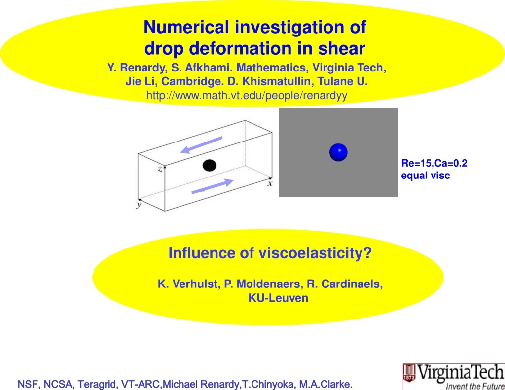
This study examines the deformation of drops in shear flow using numerical methods, with a focus on the influence of viscoelasticity. The research takes into account various parameters such as viscosity ratio, density ratio, capillary number, and Reynolds number. The governing equations for a volume-of-fluid method for Newtonian liquids are solved using finite differences on a staggered grid. The results provide valuable insights into drop deformation behavior.

E N D
Numerical investigation of drop deformation in shear Y. Renardy, S. Afkhami. Mathematics, Virginia Tech, Jie Li, Cambridge. D. Khismatullin, Tulane U. http://www.math.vt.edu/people/renardyy Re=15,Ca=0.2equal visc Influence of viscoelasticity? K. Verhulst, P. Moldenaers, R. Cardinaels, KU-Leuven NSF, NCSA, Teragrid, VT-ARC,Michael Renardy,T.Chinyoka, M.A.Clarke.
A useful way to recycle plastics is to melt and mix them to form incompatible polymer blends microstructure of HIPS. An incompatible polymer blend is a new material, combining the desired properties of the two original plastics.
A cutaway diagram shows the geometry of the device in which a drop travels in the experiments of J. Waldmeyer (PhD 2008) Waldmeyer,Mackley,Renardy,Renardy 2008 ICR The cross-section on the right shows two sample stream lines of the base flow. If the drop is small, then we can set up the boundary conditions in our simple shear flow from the strain rates of the baseflow.
The plan for this presentation Nichols, Hirt, Hotchkiss, Los Alamos Sci. Lab. Rep. LA-8355, 1980. (SOLA-VOF) Kothe, Mjolsness, Torrey, Los Alamos Nat. Lab. Rep.,1991.(RIPPLE) Brackbill, Kothe, Zemach, J. Comput. Phys.1992(CSF) Zaleski et a lJ. C Phys. 1994 SURFER,(Institut d’Alembert) Li, Renardy,Renardy Phys.Fluids 2000 • We begin with a description of the Newtonian VOF-CSF method in the context of drop deformation. • For some simulations, a higher-order method like VOF-PROST is needed. e.g. drop retraction when shearing stops. • Implementation of 3D Oldroyd B or Giesekus constitutive model. Renardy,Renardy, J C P (2002) VOF PROST Newtonian Khismatullin,Renardy,Renardy,JNNFM 2006 Giesekus Renardy,Renardy,Benyahia,Assighaou,PRE2009 2D: Hooper, de Almeida, Macosko, Derby, JNNFM, 2001 (finite element) Yue, Feng, Liu, Shen, JFM, 2005(phase field) 3D: Pillapakkam, Singh, J. Comp. Phys. 2001 (level set) Khismatullin,Renardy,Renardy JNNFM (2006) (3D) Aggarwal, Sarkar, JFM 2007. Front-tracking fin diff scheme. Hulsen et al…
The dimensionless parameters for the Newtonian case are • Viscosity ratiomhdrophmatrix • Density ratio rd/ rm • Capillary numberCahm’a/ viscous force causing deformation / capillary force which keeps the drop together. Shear rate’ (Utop-Ubottom plate )/ Lz Initial drop radiusa • Reynolds numberRe=m’ a2 / hm Interfacial tension z=Lz x=Lx y=Ly
Governing equations for a volume-of-fluid method for Newtonian liquids Fluid 1 Fluid 2 • A color function C(x,y,z,t) is advected by the flowfield • We reconstruct the interface from the surface where C jumps • Body force includes the interfacial tension force • Periodic boundary conditions in the x and y directions, and no slip at the walls z=0, z=1
Δzk Δyj Δxi The spatial discretization is a regular Cartesian grid. C(i,j,k)=0 Wijk Vijk Pijk.Cijk Uijk C(i,j,k)=1 e.g. C(i,j,k)=1/3 Finite differences are used to calculate derivatives. Staggered grid. In a cell that is cut by the interface, fluid property is averaged.
Ui-½ Ui+½ V1i,j,k V2i,j,k V3i,j,k We began with SURFER, which treats high Re flows. (open source, S. Zaleski 1997) 1. The interface is reconstructed from C(i,j,k,t) as a plane in each 3D cell, or a line in a 2D cell: C=0 C=0.7 C=1 In a cell that is cut by the interface, C = volume fraction of fluid 1. • PLIC – piecewise linear interface reconstruction • Lagrangian advection yields C at each timestep
2. VOF codes typically use the projection method on the momentum equations, and an explicit temporal discretization. Chorin 1967 • We know the solution at the nth timestep. • Next, solve for an intermediate velocity field u* without p. • Compute a correction p, using Solve with multigrid method • Solve for un+1:
The explicit time integration scheme is not feasible for low Re drop-breakup simulations. The explicit scheme is stable when Dt << time scale of viscous diffusion: mesh2 / viscosity Implicit scheme would be slow because variables are coupled large full matrix Semi-implicit scheme with decoupling of u, v,w SURFER++ Li, Renardy, Renardy 1998
The Stokes operator is associated with viscous diffusion. • We know the solution at the nth timestep. • Next, solve for an intermediate velocity field u* without p. The Stokes operator causes the need for small Dt for low Re, so treat some of this expression implicitly *
We developed and implemented a semi-implicit time integration schemeLi,Renardy,Renardy 1998 Let us take the X-component of the intermediate velocity field: The Stokes operator terms for u* are treated implicitly. =explicit terms We factorize this (Zang,Street,Koseff 1994). Finally, we invert tridiagonal matrices. Analogously for v* and w*.
3. How VOF-CSF-PLIC discretizes the interfacial tension force Fs . k = - div ns At the continuum level, At the discrete level, C=volume fraction of fluid 1 per cell. Finite differences of the discontinuous function C give ns , more finite diffs & nonlinear combinations give k .
The Continuous Surface Force Formulation (CSF) works well in an average sense for flows. • CSFBrackbill et.al 1992, Kothe,Williams,Puckett 1998,… Introduce a mollified C in Fs over a distance much larger than the mesh: where f(x,e) is a kernel. Diffusion of surface tension force? • CSS Continuous Surface Stress Formulation Lafaurie et.al 1994, Zaleski,Li,Gueyffier,…
Application: The Cambridge Shear System was used to obtain experimental data on drop deformation for oscillatory, step, & steady shear Wannaborworn, Mackley, Y. Renardy, 2002 • PDMS drop in PIB • s = 4 mN/m • = 80 Pa.s for both Equal density
VOF-CSF reproduces the initial transient for oscillatory shear experiment at 0.3Hz 250% strain 30.175 mm diameter drop. Numerical Expt
Microchannel application: 3D Newtonian Stokes flow Ca=0.4, R0/H=0.34 VOF-CSF simulation (Re=0.1) Experimental data of Sibillo, Pasquariello, Simeone, Guido, Soc. of Rheol. Meeting, 2005. Inertia is destabilizing, so add a small amount to break the drop: Re=2, Ca=0.4 Monodisperse droplets H YRenardy, Rheol Acta 2007
VOF-CSF-PLIC does not converge with spatial refinement for capillary breakup of filament. The simulation of surface-tension-dominated regimes produce small SPURIOUS CURRENTS Mesh a/8 a/12 a/16 a/20 View from top Re=12, Ca=1.14Cac
EXACT SOLUTION for all time: zero velocity. The simulation of a drop in another liquid with zero initial velocity. Prescribed surface tension Zero velocity boundary condition Discretized in the same manner as l.h.s. SPURIOUS CURRENTS :
VOF-Continuous Surface Force Formulation. Velocity vector plots across centerline in x-z plane for different mesh size at t=200Dt. Dx=a/20 Dx=a/12 Magnitudes of v increase in Lmax and L2, remain same in L1
1/96 1/128 1/160 1/192 0.0017998 0.0018409 0.0018905 0.0019688 0.0000840 0.0000854 0.0000860 0.0000863 0.0000147 0.0000154 0.0000157 0.0000157 method CSF 0.0037704 0.0038588 0.0036042 0.0039840 0.0001418 0.0001245 0.0001123 0.0001045 0.0000192 0.0000162 0.0000144 0.0000135 CSS 1/96 1/128 1/160 1/192 0.0000224 0.0000131 0.0000095 0.0000057 0.0000009 0.0000005 0.0000004 0.0000002 0.00000014 0.00000009 0.00000007 0.00000004 PROST Norms of v at 200th timestep Dt=10-5 should approach 0 as mesh-size decreases. x 1/96 1/128 1/160 1/192 O(x)2
Moral of the story you can’t win the game by finite differencing C
Δzk Δyj Δxi • Our VOF-PROST algorithm implements • A sharp interface reconstruction and Lagrangian advection of the VOF function. JCP,Renardy,Renardy 2002 • 2.A modified projection method with semi-implicit time integration is used for the momentum and constitutive equations. Li,Renardy,Renardy 1998 x0 Optimization scheme yields the mean curvaturek = 2 tr(A)at cell centers.
PROST achieves convergence of fragment volumes with mesh refinement Dx=a/12 t=22.5 Dx=a/16 t=24 Re=12
The next slides show the implementation of PROST for viscoelastic liquids
Our governing equations use the Giesekus model: Model parameter (shear-thinning) relaxation time hp Initial condition for a drop in shear: zero viscoelastic stress and impulsive startup for velocities. • We use periodic boundary conditions in the x and y directions, and no slip at the walls z=0, z=1 • An initial condition for a drop in shear is zero viscoelastic stress and impulsive startup for velocities.
Dimensionless parameters • Reynolds number smallRe=m’ a2 / hm • Density ratio 1= rd/ rm • Capillary numberCahm’a/ =viscous force deforms drop / capillary force retracts drop. • Viscosity ratiomhdrophmatrix • Weissenberg numbersWe=g ‘ l or Deborah numbers Dem= Wem(1-bm)/Ca Ded= Wed(1-bd)/(mCa) measures viscoelastic vs capillary effects. • Retardation parameterb= hsolvent / htotal • Giesekus model parameter 0<k<0.5
Positive definite property of the extra stress tensor is retained in our algorithm. The time-dependent UCM eqns have an instability if an eigenvalue of the extra stress tensor is < -G(0). (Rutkevich 1967) This does not happen if the initial data are ‘physical’, but can happen numerically. Interface cell -- Fluid properties are interpolated. -- This 'partly elastic' fluid changes properties as the interface moves, and need not satisfy the stability constraint. We correct this numerical instability by adding a multiple of Ito T over interface cells if eval < -G(0). Newtonian Viscoelastic
We use our semi-implicit time integration scheme and operator factorization for the constitutive equation -λκ(T(n))2
Our choice of implicit terms allows for the decoupling of variables followed by inversion of tridiagonal matrices T(n+1) -λκ(T(n))2 VOF-PROST runs on shared-memory machines. Mesh Dx=Dy=Dz=a/12 typically use 16 cpus, SGI Altix, 10 days. 10 million unknowns per timestep, 200,000 timesteps
3D simulations for experimental results of Moldenaers et al are shown next. BF2 (Verhulst thesis)
A Boger fluid drop in a Newtonian matrix. De_d = 1.54. Viscosity ratio 1.5, is more retracted with increased shear rate because the viscoelastic stresses at the drop tips act pull the drop in. - - - Newtonian CSF simulation ____ Oldroyd B CSF simulation Ca=0.32 o experiment Ca=0.14 Ca=0.14 Ca=0.32 Rotational flow inside the drop does not generate as much viscoelastic stress as when the fluids are reversed.
A Newtonian drop in Boger fluid matrix. De_m = 1.89, viscosity ratio 1.5, b_m=0.68,Ca=0.35, increases the initial overshoot with increase in shear rate, and retracts over a long time scale. NE-NE steady state is here. o experiment (D decreases over longer time scale) Small def. theory : D is same as NE-NE.Greco JNNFM 2002 _._. Giesekus ____ Oldroyd B Shear-thinning… smaller stresses in the VE ‘ stress wake’
A new breakup scenario for a viscoelastic drop in a Newtonian matrix was found experimentally at visc ratio 1.5 Verhulst thesis 2008 Elongation and necking to t’=100 is followed by interfacial tension forming dumbbells joined by a filament. The viscoelastic filament thins but instead of breaking, pulls the ends to coalescle. A second end-pinching elongates the drop more than in the first. Beads form on the filament. Filament breaks.
3D Numerical simulations at a higher Ca=0.65, same Ded=0.92 , forms dumbbells and a uniform filament. The dumbbells end-pinch numerically when the filament is under-resolved. Dx=R0/12 Domain 16R0x16R0x8R0 Dt=.0005/g’ 12days,16cpus,SGI Altix Experimental Large stresses build up at the neck by t’=35 and grows on the filament side. Interfacial tension forms dumbbell shape. If the filament were constrained not to break then high stresses there would pull the ends together. 1D surface tension driven breakup of an Oldroyd-B filament in vacuum never breaks. (M.Renardy 1994,1995) Does the Boger fluid remain Oldroyd-B when the filament thins a long time?
Effect of shear flow history A solution in Stokes flow does not depend on the initial condition. This uniqueness is lost when additional effects such as viscoelasticity are added (or for instance, inertia. IJMF 2008). NE-VE at visc ratio 0.75, Ca=0.5, Dem=1.54, breaks up VOF-PROST simulation with Giesekus parameter 0.1,mesh a/12. … but not when the shear rate is ramped up in small steps.
Numerical simulations with the one-mode Giesekus model with model parameter 0.1. The same level of viscoelastic stress is associated with breakup or settling The same level of viscoelastic stress occurs with breakup or settling
The End Questions?