Download
1 / 34
340 likes | 349 Views
Computational Geometry. Chapter 8 Arrangements and Duality. Minimum-Area Triangle, the problem. Given a set of n points, determine the three points that form the triangle of minimum area. On the Agenda. Duality Line Arrangements Applications. Duality. Order-Preserving Duality.

E N D
Computational Geometry Chapter 8 Arrangements and Duality
Minimum-Area Triangle,the problem Given a set of n points, determine the three points that form the triangle of minimum area.
On the Agenda • Duality • Line Arrangements • Applications
Order-Preserving Duality Note: Vertical lines (x=C, for a constant C) are not mapped by this duality (or, actually, are mapped to “points at infinity”). We ignore such lines since we can: Avoid vertical lines by a slight rotation of the plane; or Handle vertical lines separately.
Duality Properties Self-inverse: (P*)* = P , (ℓ *)* = ℓ . Incidence preserving: P ℓ ℓ * P*. 1 1 1 1 2 2 -2 1 Order preserving: P above/on/below ℓ ℓ* above/on/below P* (the point is always below/on/above the line).
Duality Properties (cont.) Points P1,P2,P3 collinear on ℓ Lines P1*, P2*, P3* intersect at ℓ *. (Follows directly from property 2.)
Duality Properties (cont.) The dual of a line segment s=[P1P2] is a double wedge that contains all the dual lines of points P on s. All these points P are collinear, therefore, all their dual lines intersect at one point, the intersection of P1* and P2*. Line ℓ intersects segment s ℓ * s*. Question: How can ℓ be located so that ℓ * appears in the right side of the double wedge? P1 P2* P ℓ ℓ * P1* P2
Minimum-Area Triangle,in the dual plane For each pair of points pi and pj (assume pipj is the triangle base): Identify the vertex v of the arrangement, corresponding to the line through these points. Find the line of the arrangement that is closest vertically to v. Remember the best line so far. Output point corresponding to the best dual line. primal pj pi y=ax+b pk y=ax+b’ pj* pi* v=(a,b) dual pk* (a,b’)
Line Arrangement • Given a set L of n lines in the plane, their arrangementA(L) is the plane subdivision induced by L. • Theorem: The combinatorial complexity of the arrangement of n lines is (n2) in the worst case. • Proof: • Number of vertices (each pair of different lines may intersect at most once). • Number of edges n2 (each line is cut into at most n pieces by at most n-1 other lines). • Number of faces (by Euler’s formula and connecting all rays to a point at infinity). Equalities hold for lines in general position. (Show!)
Line Arrangement • Goal: Compute this planar map (as a DCEL). • A plane-sweep algorithm would require (n2 log n) time (after finding the leftmost event*): (n2) events, (log n) time each. (*) Question: How can the leftmost event be found in O(n log n) time instead of O(n2) time?
An Incremental Algorithm • Input: A set L of n lines in the plane. • Output: The DCEL structure for the arrangement A(L), i.e., the subdivision induced by L in a bounding box B(L) that contains all the intersections of lines in L. • The algorithm: • Compute a bounding box B(L), and initialize the DCEL. • Insert one line after another. For each line, locate the entry face, and update the arrangement, face by face, along the path of faces (“zone”) traversed by the line.
Line Arrangement Algorithm (cont.) • After inserting the ith line, the complexity of the map is O(i2). ((i2) in the worst case—general position.) • The time complexity of each insertion of a line depends on the complexity of its zone.
Zone of a Line • The zone of a line ℓ in the arrangement A(L) is the set of faces of A(L) intersected by ℓ. • The complexity of a zone is the total complexity of all its faces: the total sum of edges (or vertices) of these faces.
The Zone Theorem • Theorem: In an arrangement of n lines, the complexity of the zone of a line is O(n). • Proof (sketch): • Consider a line ℓ. Assume without loss of generality that ℓ is horizontal. • Assume first that there are no horizontal lines. • Count the number of left bounding edges in the zone, and prove that this is at most 4n. (Same idea for right bounding edges.) ℓ3 ℓ2 ℓ4 ℓ1 ℓ
Zone Complexity: Proof • By induction on n. • For n=1: Trivial. • For n>1: • Let ℓ1 be the rightmost line intersecting ℓ (assume it’s unique). • By the induction hypothesis, the zone of ℓ in A(L\{ℓ1}) has at most 4(n-1) left bounding edges. • When adding ℓ1, the number of such edges increases: ℓ1 • One new edge on ℓ1. • Two old edges split by ℓ1. v ℓ w Hence, the new zone complexity is at most 4(n-1)+3 < 4n.
Zone Complexity: Proof (cont.) • And what happens if several lines (>2) intersect ℓ in the rightmost intersection points (i.e., if ℓ1 is not unique)? • Pick ℓ1 randomly out of these lines. • By the induction hypothesis, the zone of ℓ in A(L\{ℓ1}) has at most 4(n-1) left bounding edges. • When adding ℓ1, the number of such edges increases: • Two new edges on ℓ1. • Two old edges split by ℓ1. ℓ1 v ℓ w Hence, the new zone complexity is at most 4(n-1)+4 = 4n.
Zone Complexity: Proof (cont.) And what happens if exactly two lines intersect ℓ in the rightmost intersection points (i.e., if ℓ1 is not unique)? Denote these lines by ℓ1 ‘ℓ2 Discard both of them By the induction hypothesis, the zone of ℓ in A(L\{ℓ1‘ℓ2}) has at most 4(n-2) left bounding edges. When adding ℓ1, the number of such edges increases by at most 3 When adding ℓ2, the number of such edges increases by at most 5 ℓ1 ℓ Hence, the new zone complexity is at most 4(n-2)+3+5 = 4n. ℓ2
Zone Complexity: Proof (cont.) • And what if there are horizontal lines? • If these lines are parallel to ℓ, then just (imaginarily) rotate them; this will only increase the complexity of the zone of ℓ. • If there is a line ℓ0identical to ℓ, then the complexity of the zone of ℓ is equal to that of the zone of ℓ0. • If there are several lines identical to ℓ, their multiplicity does not increase the complexity of the zone of ℓ.
Constructing the Arrangement • The time required to insert a line ℓi is linear in the complexity of its zone, which is linear in the number of the already existing lines. Therefore, the total time is Finding a Finding According bounding box the entry to the zone (can be done point (bin. theorem in O(n log n)) search) • Note: The bound does not depend on the line-insertion order! (All orders are good.)
More on Duality
The Envelope Problem • Problem: Find the (convex) lower/upper envelope of a set of lines ℓi – the boundary of the intersection of the halfplanes lying below/above all the lines. • Theorem: Computing the lower (upper) envelope is equivalent to computing the lower (upper) convex hull of the points ℓi* in the dual plane. • Proof: Using the order-preserving property.
Parabola: Duality Interpretation • Theorem: The dual line of a point on the parabola y=x2/2 is the tangent to the parabola at that point. • Proof: • Consider the parabola y=x2/2. Its derivative is y’=x. • A point on the parabola: P(a,a2/2). Its dual: y=ax-a2/2. • Compute the tangent at P: It is the line y=cx+d passing through (a,a2/2) with slope c=a.Therefore, a2/2=a∙a+d, that is, d=-a2/2, so the line is y=ax-a2/2. y=x2/2 P(a,a2/2) y=ax-a2/2
Parabola: Duality Interpretation (cont.) • And what about points not on the parabola? • The dual lines of two points (a,b1) and (a,b2) have the same slope and the opposite vertical order with vertical distance |b1-b2|. y=x2/2 P*1: y=ax-b1 P2(a,b2) P*2: y=ax-b2 P1(a,b1)
Yet Another Interpretation ℓ1 q* ℓ2 P1 P2 Problem: Given a point q, what is q*? • Construct the two tangents ℓ1, ℓ2 to the parabola y=x2/2 that pass through q. Denote the tangency points by P1, P2. • Draw the line joining P1 and P2. This is q*! • Reason: q on ℓ1 → P1= ℓ1* on q*. q on ℓ2 → P2= ℓ2* on q*. Hence, q* = P1P2. q
Application 1: Minimum-Area Triangle • Given a set of n points*, determine the three points that form the triangle of minimum area. • Easy to solve in (n3) time, but not so easy to solve in O(n2) time. • May be solved in (n2) time using the line arrangement in the dual plane. (*) Finding the specific set of n points that maximizes the area of the minimum-area triangle is the famous Heilbronn’s triangle problem.
An (n2)-Time Algorithm primary • Construct the arrangement of dual lines in (n2) time. • For each pair of points pi and pj (assume pipj is the triangle base): • Identify the vertex v of the arrangement, corresponding to the line through these points. • Find the line of the arrangement that is closest vertically to v. • Remember the best line so far. • Output point corresponding to the best dual line. • Questions: Why is it easier to find pk* than pk? Why is it OK to look vertically? Why is the total running time only (n2)? pj pi y=ax+b pk y=ax+b’ pj* pi* v=(a,b) dual pk* (a,b’)
Application 2: Discrepancy • Given a set S of n points in the unit square U=[0,1]2. • For a given line ℓ, how many points lie below ℓ ? • Let h be the halfplane below ℓ. • If the points are well distributed, this number should be close to (h)∙n, where (h) = |U∩h|. Define S(h) = |S∩h|/|S|. • The discrepancy of S with respect to h is: S(h) = |(h)-S(h)| • The halfplane discrepancy of S is (S) = suph S(h) U S ℓ Observation: To compute (S), it suffices to consider halfplanes that pass through pairs of points. Naive algorithm: (n3) time.
Computing Discrepancy • In the dual plane, this is equivalent to counting the number of dual lines above the dual point. p q q* p* S* S
Computing Discrepancy (cont.) • For every vertex in A(S*), compute the number of lines above it, passing through it (2 in general position), or lying below it. • These three numbers sum up to n, so it suffices to compute only two of them. • From the DCEL structure we know how many lines pass through each vertex.
L1 L3 L5 Levels of an Arrangement • A point is at levelk in an arrangement of n lines if there are at most k-1 lines above this point and at most n-k lines below this point. • There are n levels in an arrangement of n lines. • A vertex can be on multiple levels, depending on the number of lines passing through it. • (Sometimes levels are counted from 0 instead of 1.)
L3 L5 An (n2)-Time Algorithm • Construct the dual arrangement. • For each line, compute the levels of all its vertices: • Compute the levels of the left infinite rays by sorting slopes. O(n log n) time. • Traverse all the lines from left to right, incrementing or decrementing the level, depending on the direction (slope) of the crossing line. (n) time for each line. • Total: (n2) time. 2 3 3 4 4 5