Download

1 / 19
190 likes | 199 Views
Alex Tabarrok. Instrumental Variables. Introduction. If an omitted variable is a determinant of Y and it is correlated with X then the fundamental requirement for regression to estimate a causal factor, , fails. What to do? Include the omitted variable!

E N D
Alex Tabarrok Instrumental Variables
Introduction • If an omitted variable is a determinant of Y and it is correlated with X then the fundamental requirement for regression to estimate a causal factor, , fails. • What to do? • Include the omitted variable! • What about if we don’t have the omitted variable and don’t even know what it might be? • Surprisingly, there is a solution.
The Search for Random Variation • Ideally we would control X randomly and run a trial. E.g. ideally we would like to determine education randomly and then find the effect of education variation on earnings. • Experiments are expensive and not always possible. • One approach is to look for “natural experiments.” • A second related approach is to note that there is a lot of variation in X. Surely some of it is due to random factors, i.e. to factors not associated with earnings. • Not every high ability student gets a PhD and not every low ability student stops at high school. Surely some of this is random? • An IV is a strategy to identify some random variation in X and use that variation and that variation alone to estimate the effect of X on Y. • A possible issue with IV is already identified. We are going to have to throw away a lot of variation to focus on the variation that is randomly determined.
Instrumental Variables • Why might education vary for a random reason (i.e. a reason not correlated with ability or other determinant of earnings)? • Some people live near a college, others do not. Someone who lives near a college may find it cheaper to go to college since they can live at home. If living near a college is random (wrt to factors like ability that determine earnings) then we can use living near a college as an IV to estimate the effect of education on earnings. • The idea of the IV is to “isolate” the variation in education that is random.
DAG: Directed Acyclic Graph • Omitted variable bias. Standard notation and DAG. U |] X Y • IV solution (2SLS). Standard notation and DAG. U Corr Instrument relevance Corr Z X Y
IV with DAG • IV solution. Standard notation and DAG. U Z X Y • The DAG is very clear on what to do. • Regress X on Z, learn (first stage) • Regress Z on Y learn (reduced form) • Divide!
IV Language • First stage—show Z influences X. • Reduced form, influence of Z on Y (intention to treat effect). • IV=Reduced Form/First Stage U Z X Y First Stage Reduced Form
Weak Instruments • DAG also makes clear why we need a strong first stage, , since • If is small we have a weak instrument and any bias will blow up . U Z X Y
Angrist-Krueger IV • Children born in December and children born in January are similar but at around age 6 the former goes to school and the latter is still in kindergarten. • Either, however, can quit at age 16 but the December quitter will have had more school at age 16 than the January (1’st QOB) quitter. Thus later QOB->more education. • Use QOB as Z to instrument for X (education) Cunningham, Mixtape.
Instruments in Action (Angrist and Krueger 1991)
Angrist-Krueger IV • Does it pass exclusion? • Weak Instruments?
Exclusion Restriction U • The exclusion restriction says that Z can influence Y only through X. • A useful way of thinking about this is to imagine that X is fixed but Z is still variable. There should be no effect on Y. • Alternatively imagine that for some Z there should be no effect on X then for these Z we should see no effect on Y. X Z Y • E.g. imagine in Angrist-Krueger that there are some states where students are not allowed to quit at 16. In these states QOB should not influence education and thus should not influence earnings. • N.B. this is testable. If QOB influenced earnings even in states where students were not allowed to quit at age 16 this would suggest a violation of exclusion. • Potential solution. Subtract the effect of QOB on earnings found in the can’t quit at age 16 sample from the can quit at age 16 sample to arrive at the true effect. • See Plausible Exogenous (Conley et al. 2012) and especially Beyond Plausibly Exogenous (Kippersluis and Rietveld 2018) for how to do this.
Mathematics of IV (2SLS) • Consider the case of one endogenous regressor and one instrument. Let the population model be: • Assume that so we cannot consistently estimate using OLS. Suppose, however, we have an instrument, Z, that satisfies the following three conditions: • Exclusion restriction follows from 1 and 2. Exclusion says Z affects Y only through X. • Monotonicity (no defiers)—instrument works in same direction for all cases.
2SLS • If our 3 conditions are satisfied we can estimate using the following two stage procedure. First regress X on Z. • This regression “decomposes” X into two parts. The part that can be predicted from Z, , and the error component. • Since Z is not correlated with u the part of X that is predicted by Z, ,won’t be correlated with u either. • Thus we can consistently estimate by by regressing Y on the predicted X: The First Stage Equation
2SLS in STATA • ivregress 2sls Y exogvarlist (endogvar=IV var), vce(robust) • Follow by “estatfirststage” • With more than one instrument • ivregress 2sls Y exogvarlist (endogvar=IV1 IV2), vce(robust) • Follow by “estate overid” to check for consistency.
IV with Two Binary Variables (interesting special case) • We are interested in effect of treatment, T[0,1] on outcome Y. • But suppose T is correlated with other unobserved variables that also affect Y. • We find a Z that satisfies IV assumptions. • Notice that when Z=1 the probability of T=1 increases by .45. • Now consider . Since by exclusionassumption the only reason why Z changes Y is the influence on T this must be the due to the influence of a probabilistic increase in T of .45. • Thus true influence of T going from 0 to 1 is:
IV with Two Binary Variables • Assume • Then .75 of the observations with will have outcomes of • .25 of the observations with will have outcomes of • .3 of the obs with will have outcomes of • .7 of the obs with will have outcomes of • Let’s now write out
IV with Two Binary Variables (Wald Estimator) =.45 • More generally
Finding Good Instruments • Art more than science. Key is to know details, details, details about your area of research. • Creativity: e.g. Levitt and effect of police on crime. • Some common sources: • Probabilities may be assigned randomly even when treatments are not. Encouragement designs. • Distances. • Policy reforms. • Random variation in assignment (judges)