Download

1 / 18
180 likes | 346 Views
Landmark Classification in Large-scale Image Collections. Yunpeng Li David J. Crandall Daniel P. Huttenlocher ICCV 2009. Outline. Introduction Building Internet-Scale Datasets Image Classification Experiments Conclusion. Introduction. Goal

E N D
Landmark Classification in Large-scale Image Collections Yunpeng Li David J. Crandall Daniel P. Huttenlocher ICCV 2009
Outline • Introduction • Building Internet-Scale Datasets • Image Classification • Experiments • Conclusion
Introduction • Goal • Image classification on much larger datasets featuring millions of images and hundreds of categories • Image classification • Multiclass SVM • Flickr • landmark • Geotagged photos • Text tag
Building Internet-Scale Datasets • Long-term goal • to create large labeled datasets • To retrieve Flickr60 million geotaggedphotos • x, y coordinates • Eliminate photos • (worse than about a city block) -> 30 million photos • Mean shift cluster • radius of the disc is about 100m[3] • Peaks in the photo density distribution[5] • at most 5 photos from any given Flickr user towards any given peak • Top 500 peaks as categories • 500th peak has 585 photos • 1000th peak has 284 photos • Final Dataset 1.9 million photos
Image Feature(visual) Visualword Clustering SIFT descriptors from photos in the training set k-means Approximate nearest neighbor(ANN)[1] Form a frequency vector which counts the number of occurrences of each visual word in the image Normalize L2-norm of 1
Image Feature(text tag) At least 3 different users Binary vector indicate presence or absence Normalize L2-norm of 1
Image Feature(Combination) Normalize L2-norm of 1
Image Classification • Find which class has the highest score • m is the number of classes • x is the feature vector of an image • is the weighting model • is the score for class y under w • It’s by nature a multiway(as opposed to binary) classification problem
Image Classification • Multiclass SVM[4] to learn model w • Using the SVM software package[9] • A set of training examples • Multiclass SVM optimize the objective function
Experiments(1/6) • Dataset 2 million images • Each of these experiments evenly divided the dataset into test and training image sets • The number of images used in an m-way classification experiment, the baseline probability of a correct random guess is 1/m.
Experiments(4/6) • 20 well-traveled people to each label 50 photos taken at the world’s top ten landmarks. • Textual tags were also shown for a random subset of the photos. • the average human classification accuracy was 68.0% without textual tags and 76.4% when both the image and tags were shown • Thus the humans performed better than the automatic classifier when using visual features alone (68.0% versus 57.55%) but about the same when both text and visual features were available (76.4% versus 80.91%).
Experiments(5/6) • Visual vocabulary K 20% 50%
Experiments(6/6) • Image classification on a single 2.66 GHz cpu • total time 2.4s • most of which is consumed by SIFT interest point detection • If SIFT features are extracted, classification requires only • 3.06 ms for 200 categories • 0.15 ms for 20 categories
Conclusion • Creating large labeled image datasets from geotagged image collections, which nearly 2 million are labeled. • Demonstrate multiclass SVM classifiers using SIFT-based bag-of-word featuresachieve quite good classification rates for largescale problems, with accuracy that in some cases is comparable to that of humans on the same task. • With text features from tagging, the accuracy can be hundreds of times the baseline.