Download
1 / 39
390 likes | 523 Views
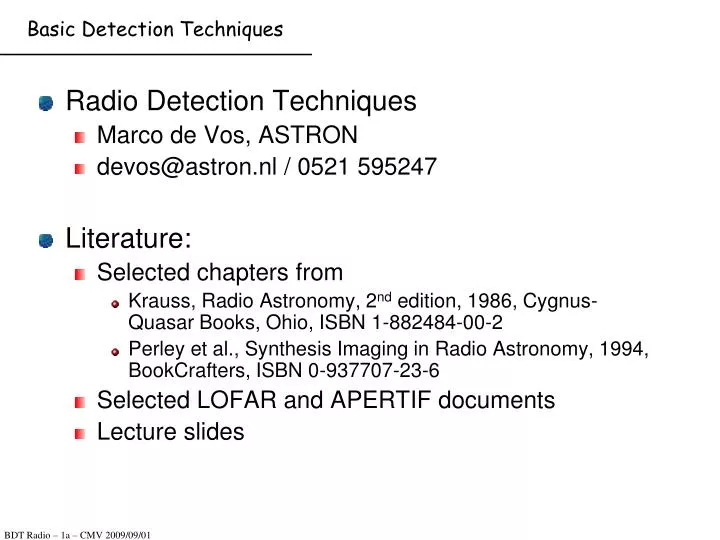
Basic Detection Techniques. Radio Detection Techniques Marco de Vos, ASTRON devos@astron.nl / 0521 595247 Literature: Selected chapters from Krauss, Radio Astronomy, 2 nd edition, 1986, Cygnus-Quasar Books, Ohio, ISBN 1-882484-00-2

E N D
Basic Detection Techniques • Radio Detection Techniques • Marco de Vos, ASTRON • devos@astron.nl / 0521 595247 • Literature: • Selected chapters from • Krauss, Radio Astronomy, 2nd edition, 1986, Cygnus-Quasar Books, Ohio, ISBN 1-882484-00-2 • Perley et al., Synthesis Imaging in Radio Astronomy, 1994, BookCrafters, ISBN 0-937707-23-6 • Selected LOFAR and APERTIF documents • Lecture slides
Overview • 1a (2011/09/20): Introduction and basic properties • Historical overview, detection of 21cm line, major telescopes, SKA • Basis properties: coherent detection, sensitivity, resolution • 1b (2011/09/22 TBC): Single dish systems • Theory: basic properties, sky noise, system noise, Aeff/Tsys, receiver systems, mixing, filtering, A/D conversion • Case study: pulsar detection with the Dwingeloo Radio Telescope • 2a (2011/09/26): Aperture synthesis arrays • Theory: correlation, aperture synthesis, van Cittert-Zernike relation, propagation of instrumental effects • Case study: imaging with the WSRT • 2b (2011/09/27): Phase array systems • Theory: aperture arrays and phased arrays, feed properties, sensitivity, calibration. • Case study: the LOFAR system • Experiment (2011/09/29 TBC): Phased Array Feed flux measurement • Measurements with DIGESTIF (in Dwingeloo)
Coherent detectors • Responds to electric field ampl. of incident EM waves • Active dipole antenna • Dish + feed horn + LNA • Requires full receiver chain, up to A/D conversion • Radio • mm (turnoverpoint @ 300K) • IR (downconversion by mixing with laser LOs) • Phase is preserved • Separation of polarizations • Typically narrow band • But tunable, and with high spectral resolution • For higher frequencies: needs frequency conversion schemes
“Unique selling points” of radio astronomy • Technical: • Radio astronomy works at the diffraction limit (/D) • It usually works at ‘thermal noise’ limit (after ‘selfcalibration’ in interferometry) • Imaging on very wide angular resolution scales (degrees to ~100 arcsec) • Extremely energy sensitive (due to large collecting area and low photon energy) • Very wide frequency range (~5 decades; protected windows ! RFI important) • Very high spectral resolution (<< 1 km/s) achievable due to digital techniques • Very high time resolution (< 1 nanoseconds) achievable • Good dynamic range for spatial, temporal and spectral emission • Astrophysical: • Most important source of information on cosmic magnetic fields • No absorption by dust => unobscured view of Universe • Information on very hot (relativistic component, synchrotron radiation) • Diagnostics on very cold - atomic and molecular - gas
Early days of radio astronomy 1932 Discovery of cosmic radio waves (Karl Jansky) v=25MHz; dv=26kHz Galactic centre
The first radio astronomer (Grote Reber, USA) • Built the first radio telescope • "Good" angular resolution • Good visibility of the sky • Detected Milky Way, Sun, other radio sources • (ca. 1939-1947). • Published his results in astronomy journals. • Multi-frequency observations 160 & 480 MHz
Radio Spectral-lines • Predicted by van der Hulst (1944):discrete 1420 MHz (21 cm) emission from neutral Hydrogen (HI). • Detected by Ewen & Purcell (1951)
Giant radio telescopes of the world • 1957 76m Jodrell Bank, UK • ~1970 64-70m Parkes, Australia • ~1970 100m Effelsberg, Germany • ~1970 300m Arecibo, Puerto Rico • ~2000 100m GreenBank Telescope (GBT), USA
EVLA • 27 x 25m dish
Square Kilometre Array 2500 Dishes Dense Aperture Arrays 3-Core Central Region Wide Band Single Pixel Feeds 250 Sparse Aperture Arrays Phased Array Feeds 18
SKA1 baseline design 250 x 15-m dishes Baseline technologies are mature and demonstrated in the SKA Precursors and Pathfinders Central Region Single pixel feed Sparse Aperture Array stations (5 x LOFAR) 21 Artist renditions from Swinburne Astronomy Productions
EM waves • Directionality (RA, dec, spatial resolution) • Time (timing accuracy, time resolution) • Frequency (spectral resolution) • Flux (total intensity, polarization properties)
Sensitivity • Key question: • What’s the weakest source we can observe • Key issues: • Define brightness of the source • Define measurement process • Define limiting factors in that process
Brightness function • Surface brightness: • Power received /area /solid angle /bandwidth • Unit: W m-2 Hz-1 rad-2 • Received power: • Power per unit bandwidth: • Power spectrum: w(v) • Total power: • Integral over visible sky and band • Visible sky: limited by aperture • Band: limited by receiver
Point sources, extended sources • Point source: size < resolution of telescope • Extended source: size > resolution of telescope • Continuous emission: size > field of view • Flux density: • Unit: 1 Jansky (Jy) = 10-26 W m-2 Hz-1
Antenna temperature, system temperature • Express noise power received by antenna in terms of temperature of resistor needed to make it generate the same noise power. • Spectral power: w = kT/λ2 AeffΩa = kT • Observed power: W = kT Δv • Observed flux density: S = 2kT / Aeff • Tsys = Tsky + Trec • Tsky and Tant: what’s in a name • After integration:
System Equivalent Flux Density • What’s in Tsys? • 3K background and Galactic radio emission Tbg • Atmospheric emission Tsky • Spill-over from the ground and other directions Tspill • Losses in feed and input waveguide Tloss • Receiver electronics Trx • At times: calibration source Tcal
Reception pattern of an antenna • Beam solid angle (A = A/A0) • Measure of Field of View • Antenna theory: A0 Ωa = λ2
Timing • Rubidium (Rb) laser reduces variance in the GPS-PPS to < 4 ns rms over 105 sec. • The output of the Rb reference is distributed to the Time Distribution Sub-rack (TDS). • Reference frequency is converted to the sampling frequency: using 10 MHz reference and Phase Locked Loops (PLL) in combination with a Voltage Controlled Crystal Oscillator (VCXO), the jitter of the output clock signals are minimized. • Within a sub-rack all clock distribution is done differentially to reduce noise picked up by the clock traces and to reduce Electro Magnetic Interference (EMI) by the clock.