Download
1 / 19
230 likes | 625 Views
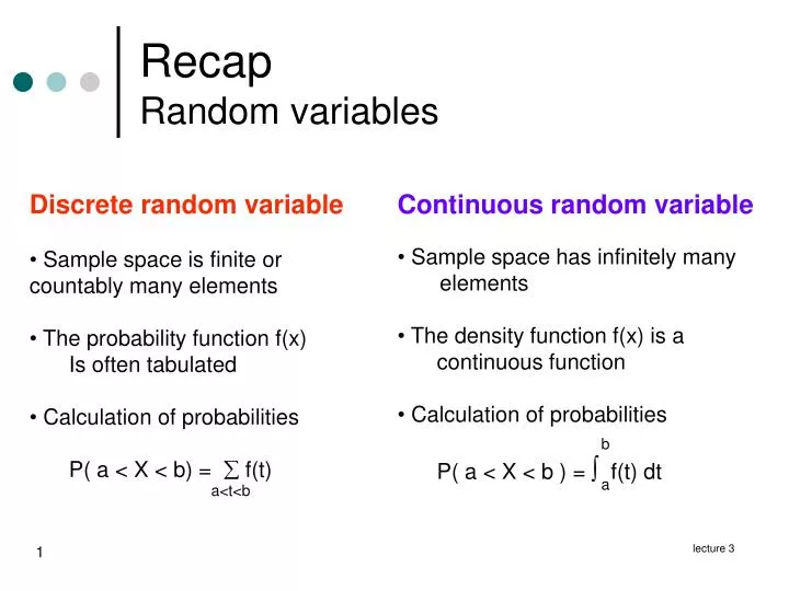
Recap Random variables. Discrete random variable Sample space is finite or countably many elements The probability function f(x) Is often tabulated Calculation of probabilities P( a < X < b) = f(t). Continuous random variable Sample space has infinitely many

E N D
RecapRandom variables • Discrete random variable • Sample space is finite or countably many elements • The probability function f(x) • Is often tabulated • Calculation of probabilities • P( a < X < b) = f(t) • Continuous random variable • Sample space has infinitely many • elements • The density function f(x) is a • continuous function • Calculation of probabilities • P( a < X < b ) = f(t) dt b a a<t<b lecture 3
Mean / Expected value Definition • Definition: • Let X be a random variable with probability / • Density function f(x). The mean or expected value of X is give by • if X is discrete, and • if X is continuous. lecture 3
Mean / Expected value Interpretation Interpretation: The total contribution of a value multiplied by the probability of the value – a weighted average. Example: Mean value= 1,5 f(x) 0.4 0.3 0.2 0.1 x 0 1 2 3 lecture 3
Mean / Expected valueExample • Problem: • A private pilot wishes to insure his plane valued at 1 mill kr. • The insurance company expects a loss with the following probabilities: • Total loss with probability 0.001 • 50% loss with probability 0.01 • 25% loss with probability 0.1 • 1. What is the expected loss in kroner ? • 2. What premium should the insurance company • ask if they want an expected profit of 3000 kr ? lecture 3
Mean / Expected value Function of a random variable • Theorem: • Let X be a random variable with probability / density function f(x). The expected value of g(X) is • if X is discrete, and • if X is continuous. lecture 3
Expected valueLinear combination • Theorem: Linear combination • Let X be a random variable (discrete or continuous), and let a and b be constants. For the random variable aX + b we have • E(aX+b) = aE(X)+b lecture 3
Mean / Expected valueExample • Problem: • The pilot from before buys a new plane valued at 2 mill kr. • The insurance company’s expected losses are unchanged: • Total loss with probability 0.001 • 50% loss with probability 0.01 • 25% loss with probability 0.1 • 1. What is the expected loss for the new plane? lecture 3
Mean / Expected valueFunction of a random variables • Definition: • Let X and Y be random variables with joint probability / density function f(x,y). The expected value of g(X,Y) is • if X and Y are discrete, and • if X and Y are continuous. lecture 3
Mean / Expected valueFunction of two random variables • Problem: • Burger King sells both via “drive-in” and “walk-in”. • Let X and Y be the fractions of the opening hours that “drive-in” and “walk-in” are busy. • Assume that the joint density for X and Y are given by f(x,y) ={ 4xy 0 x 1 , 0 y 1 0 otherwise • The turn over g(X,Y) on a single day is given by • g(X,Y) = 6000 X + 9000Y • What is the expected turn over on a single day? lecture 3
Mean / Expected value Sums and products Theorem: Sum/Product Let X and Y be random variables then E[X+Y] = E[X] + E[Y] If X and Y are independent then E[X Y] = E[X] E[Y] . . lecture 3
VarianceDefinition • Definition: • Let X be a random variable with probability / density function f(x) and expected value . The variance of X is then given • if X is discrete, and • if X is continuous. The standard deviationis the positive root of the variance: lecture 3
VarianceInterpretation The variance expresses, how dispersed the density / probability function is around the mean. Varians = 0.5 Varians = 2 f(x) f(x) 0.5 0.5 0.4 0.4 0.3 0.3 0.2 0.2 0.1 0.1 x x 1 2 3 0 1 2 3 4 Rewrite of the variance: lecture 3
VarianceLinear combinations Theorem: Linear combination Let X be a random variable, and let a be b constants. For the random variable aX + b the variance is • Examples: • Var (X + 7) = Var (X) • Var (-X ) = Var (X) • Var ( 2X ) = 4 Var (X) lecture 3
CovarianceDefinition • Definition: • Let X and Y be to random variables with joint probability / density function f(x,y). The covariancebetween X and Y is • if X and Y are discrete, and • if X and Y are continuous. lecture 3
CovarianceInterpretation • Covariance between X and Y expresses how X and Y influence each other. • Examples: Covariance between • X = sale of bicycle and Y = bicycle pumps is positive. • X = Trips booked to Spain and Y = outdoor temperature is negative. • X = # eyes on red dice and Y = # eyes on the green dice is zero. lecture 3
CovarianceProperties Theorem: The covariancebetween two random variables X and Y with means XandY, respectively, is Notice! Cov (X,X) = Var (X) If X and Y are independent random variables, then Cov (X,Y) = 0 Notice! Cov(X,Y) = 0 does not imply independence! lecture 3
Variance/CovariaceLinear combinations Theorem: Linear combination Let X and Y be random variables, and let a and b be constants. For the random variables aX + bY the variance is Specielt: Var[X+Y] = Var[X] + Var[Y] +2Cov (X,Y) If X and Y are independent, the variance is Var[X+Y] = Var[X] + Var[Y] lecture 3
CorrelationDefinition Definition: Let X and Y be two random variables with covariance Cov (X,Y) and standard deviations Xand Y, respectively. The correlation coefficient of X and Y is It holds that If X and Y are independent, then lecture 3
Mean, variance, covariaceCollection of rules Sums and multiplications of constants: E (aX) = a E(X) Var(aX) = a2Var (X) Cov(aX,bY) = abCov(X,Y) E (aX+b) = aE(X)+b Var(aX+b) = a2 Var (X) Sum: E (X+Y) = E(X) + E(Y) Var(X+Y) = Var(X) + Var(Y) + 2Cov(X,Y) X and Y are independent: E(XY) = E(X) E(Y) Var(X+Y) = Var(X) + Var(Y) lecture 3