Download
1 / 123
1.23k likes | 1.24k Views
Discover the power and applications of graphs in this introduction to graph theory. Learn about vertices, edges, connectivity, and more. Suitable for beginners.

E N D
Fonts: MTExtra: (comment) Symbol: Wingdings: Graphs 6-Graphs
What’s a Graph? • A bunch of vertices connected by edges. vertex 2 1 3 4 edge 6-Graphs
Why Graph Algorithms? • They’re fun. • They’re interesting. • They have surprisingly many applications. 6-Graphs
Graphs are Everywhere 6-Graphs
Adjacency as a Graph • Each vertex represents a state, country, etc. • There is an edge between two vertices if the corresponding areas share a border. WY NE CO KS 6-Graphs
When a Graph? • Graphs are a good representation for any collection of objects and binary relation among them: • - The relationship in space of places or objects • - The ordering in time of events or activities • - Family relationships • - Taxonomy (e.g. animal - mammal - dog) • - Precedence (x must come before y) • - Conflict (x conflicts or is incompatible with y) • - Etc. 6-Graphs
Graphs • Graph consists of two sets: set V of vertices and set E of edges. • Terminology: endpoints of the edge, loop edges, parallel edges, adjacent vertices, isolated vertex, subgraph, bridge edge • Directed graph (digraph) has each edge as an ordered pair of vertices 6-Graphs
Basic Concepts • A graph is an ordered pair (V, E). • V is the set of vertices. (You can think of them as integers 1, 2, …, n.) • E is the set of edges. An edge is a pair of vertices: (u, v). • Note: since E is a set, there is at most one edge between two vertices. (Hypergraphs permit multiple edges.) • Edges can be labeled with a weight: 10 6-Graphs
Concepts: Directedness • In a directed graph, the edges are “one-way.” So an edge (u, v) means you can go from u to v, but not vice versa. • In an undirected graph, there is no direction on the edges: you can go either way. (Also, no self-loops.) a self-loop 6-Graphs
Concepts: Adjacency • Two vertices are adjacent if there is an edge between them. • For a directed graph, u is adjacent to v iff there is an edge (v, u). v v u w u w u is adjacent to v. v is adjacent to u and w. w is adjacent to v. u is adjacent to v. v is adjacent to w. 6-Graphs
Special Graphs • Simple graph is a graph without loop or parallel edges • A complete graph of n vertices Kn is a simple graph which has an edge between each pair of vertices • A complete bipartite graph of (n, m) vertices Kn,m is a simple graph consisting of vertices, v1, v2, …, vm and w1, w2, …, wn with the following properties: • There is an edge from each vertex vi to each vertex wj • There is no edge from any vertex vi to any vertex vj • There is no edge from any vertex wi to any vertex wj 6-Graphs
Concepts: Degree • Undirected graph: The degree of a vertex is the number of edges touching it. • For a directed graph, the in-degree is the number of edges entering the vertex, and the out-degree is the number leaving it. The degree is the in-degree + the out-degree. degree 4 in-degree 2, out-degree 1 6-Graphs
Paths and Circuits • A walk in a graph is an alternating sequence of adjacent vertices and edges • A path is a walk that does not contain a repeated edge • Simple path is a path that does not contain a repeated vertex • A closed walk is a walk that starts and ends at the same vertex • A circuit is a closed walk that does not contain a repeated edge • A simple circuit is a circuit which does not have a repeated vertex except for the first and last 6-Graphs
Concepts: Path • A path is a sequence of adjacent vertices. The length of a path is the number of edges it contains, i.e. one less than the number of vertices. • We write u v if there is path from u to v. (The correct symbol, a wiggly arrow, is not available in standard fonts.) We say v is reachable from u. Is there a path from 1 to 4? What is its length? What about from 4 to 1? How many paths are there from 2 to 3? From 2 to 2? From 1 to 1? 2 1 3 4 6-Graphs
Concepts: Cycle • A cycle is a path of length at least 1 from a vertex to itself. • A graph with no cycles is acyclic. • A path with no cycles is a simple path. • The path <2, 3, 4, 2> is a cycle. 2 1 3 4 6-Graphs
Concepts: Connectedness • An undirected graph is connected iff there is a path between any two vertices. • The adjacency graph of U.S. states has three connected components. Name them. • (We say a directed graph is strongly connected iff there is a path between any two vertices.) An unconnected graph with three connected components. 6-Graphs
Connectedness • Two vertices of a graph are connected when there is a walk between two of them. • The graph is called connected when any pair of its vertices is connected • If graph is connected, then any two vertices can be connected by a simple path • If two vertices are part of a circuit and one edge is removed from the circuit then there still exists a path between these two vertices • Graph H is called a connected component of graph G when H is a subgraph of G, H is connected and H is not a subgraph of any bigger connected graph • Any graph is a union of connected components 6-Graphs
Euler Circuit • Euler circuit is a circuit that contains every vertex and every edge of a graph. Every edge is traversed exactly once. • If a graph has Euler circuit then every vertex has even degree. If some vertex of a graph has odd degree then the graph does not have an Euler circuit • If every vertex of a graph has even degree and the graph is connected then the graph has an Euler circuit • A Euler path is a path between two vertices that contains all vertices and traverces all edge exactly ones • There is an Euler path between two vertices v and w iff vertices v and w have odd degrees and all other vertices have even degrees 6-Graphs
Hamiltonian Circuit • Hamiltonian circuit is a simple circuit that contains all vertices of the graph (and each exactly once) • Traveling salesperson problem 6-Graphs
Concepts: Trees • A free tree is a connected, acyclic, undirected graph. • To get a rooted tree (the kind we’ve used up until now), designate some vertex as the root. • If the graph is disconnected, it’s a forest. • Facts about free trees: • |E| = |V| -1 • Any two vertices are connected by exactly one path. • Removing an edge disconnects the graph. • Adding an edge results in a cycle. 6-Graphs
Rooted Trees • Rooted tree is a tree in which one vertex is distinguished and called a root • Level of a vertex is the number of edges between the vertex and the root • The height of a rooted tree is the maximum level of any vertex • Children, siblings and parent vertices in a rooted tree • Ancestor, descendant relationship between vertices 6-Graphs
Binary Trees • Binary tree is a rooted tree where each internal vertex has at most two children: left and right. Left and right subtrees • Full binary tree • Representation of algebraic expressions • If T is a full binary tree with k internal vertices then T has a total of 2k + 1 vertices and k + 1 of them are leaves • Any binary tree with t leaves and height h satisfies the following inequality: t 2h 6-Graphs
Spanning Trees • A subgraph T of a graph G is called a spanning tree when T is a tree and contains all vertices of G • Every connected graph has a spanning tree • Any two spanning trees have the same number of edges • A weighted graph is a graph in which each edge has an associated real number weight • A minimal spanning tree (MST) is a spanning tree with the least total weight of its edges 6-Graphs
Graph Size • We describe the time and space complexity of graph algorithms in terms of the number of vertices, |V|, and the number of edges, |E|. • |E| can range from 0 (a totally disconnected graph) to |V|2 (a directed graph with every possible edge, including self-loops). • Because the vertical bars get in the way, we drop them most of the time. E.g. we write Q(V + E) instead of Q(|V| + |E|). 6-Graphs
2 1 3 4 Representing Graphs • Adjacency matrix: if there is an edge from vertex i to j, aij = 1; else, aij = 0. • Space: Q(V2) • Adjacency list: Adj[v] lists the vertices adjacent to v. • Space: Q(V+E) Adj: 1 2 4 2 3 3 4 4 2 Represent an undirected graph by a directed one: 6-Graphs
Depth-First Search • A way to “explore” a graph. Useful in several algorithms. • Remember preorder traversal of a binary tree? • Binary-Preorder(x):1 number x2 Binary-Preorder(left[x])3 Binary-Preorder(right[x]) • Can easily be generalized to trees whose nodes have any number of children. • This is the basis of depth-first search. We “go deep.” 1 2 5 3 4 6 7 6-Graphs
DFS on Graphs • The wrong way: • Bad-DFS(u)1 number u2 for each v in Adj[u] do3 Bad-DFS(v) • What’s the problem? 1 2 5 3 4 6 7 6-Graphs
Fixing Bad-DFS • We’ve got to indicate when a node has been visited. • Following CLRS, we’ll use a color: • WHITE never seen • GRAY discovered but not finished (still exploring its descendants) • BLACK finished 6-Graphs
A Better DFS • initially, all vertices are WHITE • Better-DFS(u) • color[u] GRAY • number u with a “discovery time” • for each v in Adj[u] do • if color[v] = WHITE then avoid looping! • Better-DFS(v) • color[u] BLACK • number u with a “finishing time” 6-Graphs
Depth-First Spanning Tree • As we’ll see, DFS creates a tree as it explores the graph. Let’s keep track of the tree as follows (actually it creates a forest not a tree): • When v is explored directly from u, we will make u the parent of v, by setting the predecessor, aka, parent () field of v to u: u u v v p[v] u 6-Graphs
Two More Ideas • 1. We will number each vertex with discovery and finishing times—these will be useful later. • The “time” is just a unique, increasing number. • The book calls these fields d[u] and f[u]. • 2. The recursive routine we’ve written will only explore a connected component. We will wrap it in another routine to make sure we explore the entire graph. 6-Graphs
graphs from p. 1081 6-Graphs
show strongly connected comps see next slide 6-Graphs
from prev slide 6-Graphs
DFS examples On an undirected graph, any edge that is not a “tree” edge is a “back” edge (from descendant to ancestor). 6-Graphs
DFS Examples 6-Graphs
DFS Example: digraph Here, we get a forest (two trees). B = back edge (descendant to ancestor, or self-loop) F = forward edge (ancestor to descendant) C = cross edge (between branches of a tree, or between trees) 6-Graphs
DFS running time is Θ(V+E) we visit each vertex once; we traverse each edge once 6-Graphs
applications of DFS Connected components of an undirected graph. Each call to DFS_VISIT (from DFS) explores an entire connected component (see ex. 22.3-11). So modify DFS to count the number of times it calls DFS_VISIT: 5 for each vertex u Є V[G] 6 do if color[u] = WHITE 6.5 then cc_counter ← cc_counter + 1 7 DFS_VISIT(u) Note: it would be easy to label each vertex with its cc number, if we wanted to (i.e. add a field to each vertex that would tell us which conn comp it belongs to). 6-Graphs
Applications of DFS Cycle detection: Does a given graph G contain a cycle? Idea #1: If DFS ever returns to a vertex it has visited, there is a cycle; otherwise, there isn’t. OK for undirected graphs, but what about: No cycles, but a DFS from 1 will reach 4 twice. Hint: what kind of edge is (3, 4)? 6-Graphs
Cycle detection theorem • Theorem: A graph G (directed or not) contains a cycle if and only if a DFS of G yields a back edge. • →: Assume G contains a cycle. Let v be the first vertex reached on the cycle by a DFS of G. All the vertices reachable from v will be explored from v, including the vertex u that is just “before” v in the cycle. Since v is an ancestor of u, the edge (u,v) will be a back edge. • ←: Say the DFS results in a back edge from u to v. Clearly, u→v (that should be a wiggly arrow, which means, “there is a path from u to v”, or “v is reachable from u”). And since v is an ancestor of u (by def of back edge), v→u (again should be wiggly). So v and u must be part of a cycle. QED. 6-Graphs
Back Edge Detection • How can we detect back edges with DFS? For undirected graphs, easy: see if we’ve visited the vertex before, i.e. color≠ WHITE. • For directed graphs: Recall that we color a vertex GRAY while its adjacent vertices are being explored. If we re-visit the vertex while it is still GRAY, we have a back edge. • We blacken a vertex when its adjacency list has been examined completely. So any edges to a BLACK vertex cannot be back edges. 6-Graphs
TOPOLOGICAL SORT “Sort” the vertices so all edges go left to right. 6-Graphs
TOPOLOGICAL SORT For topological sort to work, the graph G must be a DAG (directed acyclic graph). G’s undirected version (i.e. the version of G with the “directions” removed from the edges) need not be connected. Theorem: Listing a dag’s vertices in reverse order of finishing time (i.e. from highest to lowest) yields a topological sort. Implementation: modify DFS to stick each vertex onto the front of a linked list as the vertex is finished. see examples next slide.... 6-Graphs
Topological Sort Examples 6-Graphs
More on Topological Sort • Theorem (again): Listing a dag’s vertices in order of highest to lowest finishing time results in a topological sort. Putting it another way: If there is an edge (u,v), then f[u] > f[v]. • Proof : Assume there is an edge (u,v). • Case 1: DFS visits u first. Then v will be visited and finished before u is finished, so f[u] > f[v]. • Case 2: DFS visits v first. There cannot be a path from v to u (why not?), so v will be finished before u is even discovered. So again, f[u] > f[v]. • QED. 6-Graphs
Introduction • Start with a connected, undirected graph, and add real-valued weights to each edge. • The weights could indicate time, distance, cost, capacity, etc. 6 5 1 5 5 3 2 6 4 6 6-Graphs
Definitions • A spanning tree of a graph G is a tree that contains every vertex of G. • The weight of a tree is the sum of its edges’ weights. • A minimal spanning tree is a spanning tree with lowest weight. (The left tree is not minimal. The right one is, as we will see.) 6 5 6 5 1 1 5 5 5 5 3 2 3 2 6 4 6 4 6 6 weight = 21 weight = 15 6-Graphs