Download
1 / 32
320 likes | 603 Views
Introduction to Sequence Analysis. Utah State University – Spring 2012 STAT 5570: Statistical Bioinformatics Notes 6.1. References. Chapters 2 & 7 of Biological Sequence Analysis (Durbin et al., 2001). Review.

E N D
Introduction to Sequence Analysis Utah State University – Spring 2012 STAT 5570: Statistical Bioinformatics Notes 6.1
References • Chapters 2 & 7 of Biological Sequence Analysis (Durbin et al., 2001)
Review • Genes are:- sequences of DNA that “do” something- can be expressed as a string of: nucleic acids: A,C,G,T (4-letter alphabet) • Central Dogma of Molecular Biology DNA mRNA protein bio. action • Proteins can be expressed as a string of: amino acids: (20-letter alphabet) (sometime 24 due to “similarities”)
Why look at protein sequence? • Levels of protein structure • Primary structure: order of amino acids • Secondary structure: repeating structures (beta-sheets and alpha-helices) in “backbone” • Tertiary structure: full three-dimensional folded structure • Quartenary structure: interaction of multiple “backbones” • Sequence shape function • Similar sequence similar function -?
Consider simple pairwise alignment • Sequence 1: HEAGAWGHEE • Sequence 2: PAWHEAE • How similar are these two sequences? • Match up exactly? • Subsequences similar? • Which positions could be possibly matched without severe penalty? • To find the “best” alignment, need some way to: rate alignments
Possible alignments Sequence 1: HEAGAWGHEE Sequence 2: PAWHEAE Alignment 1: HEAGAWGHEE PAWHEAE Alignment 2: HEAGAWGHEE PAW-HE-AE Alignment 3: HEA-GAWGHEE PAWHEAE Alignment 4: HEAGAWGHE-E PAW-HEAE Think of gaps in alignment as: mutational insertion or deletion
Basic idea of scoring potential alignments • + score: identities and “conservative” substitutions • - score: non- “conservative” changes - (not expected in “real” alignments) • Add score at each position • Equivalent to assuming mutations are: independent • Reasonable assumption for DNA and proteins but not structural RNA’s
Some Notation assume independence of sequences assume residues a & b are aligned as a pair with prob. Pab
Compare these two models log likelihood ratio of pair (a,b) occurring as aligned pair, as opposed to unaligned pair
Score Matrix – or “substitution matrix” A R N D ... Y V A | 5 -2 -1 -2 -2 0 R | -2 7 -1 -2 -1 3 N | -1 -1 7 ... D | -2 -2 ... ... | s(a,b) Y | -2 -1 ... V | 0 3 These are scaled and rounded log-odds values(for computational efficiency) This is a portion of the BLOSUM50 substitution matrix; others exist.
How to get these substitution values? Basic idea: • Look at existing, “known” alignments • Compare sequences of aligned proteins and look at substitution frequencies • This is a chicken-or-the-egg problem: - alignment - - scoring scheme - Maybe better to base alignment on: tertiary structures (or some other alignment)
Some substitution matrix types • BLOSUM (Henikoff) • BLOCK substitution matrix • derived from BLOCKS database – set of aligned ungapped protein families, clustered according to threshold percentage (L) of identical residues – compare residue frequencies between clusters • L=50 BLOSUM50 • PAM (Dayhoff) • percentage of acceptable point mutations per 108 years • derived from a general model for protein evolution, based on number L of PAMs (evolutionary distance) • PAM1 from comparing sequences with <1% divergence • L=250 PAM250 = PAM1^250
Which substitution matrix to use? • No universal “best” way • In general: • low PAM find short alignments of similar seq. • high PAM find longer, weaker local alignments • BLOSUM standards: • BLOSUM50 for alignment with gaps • BLOSUM62 for ungapped alignments • higher PAM, lower BLOSUM more divergent (looking for more distantly related proteins) • A reasonable strategy: BLOSUM62 complemented with PAM250
Which matrix for aligning DNA sequences? • The BLOSUM and PAM matrices are based on similarities between amino acids –- no such similarity assumed for nucleic acids; residues either match or they don’t • Unitary matrix: identity matrix +1 for identical match – (or +3 or …) 0 for non-match – (or -2 or …)
How to score gaps? One way: affine gap penalty linear transformation followed by a translation gap opening penalty gap extension penalty(e < d) length of gap Think of gaps in alignment as: mutational insertion or deletion
start with 0 H E A G A W G H E E 0 P |A |W |H |E |A |E | begin (or continue) gap: -d (or -e) match letters (residues): + s(a,b) Tabular representation of alignment Fill in table to give max. of possible values at each successive element – keep track of which direction generated max. – then use the “path” that gives highest final score (lower right corner)
Alignment algorithms • Global: Needleman-Wunsch- find optimal alignment for entire sequences (prev. slide) • Local: Smith-Waterman- find optimal alignment for subsequences • Repeated matches- allow for starting over sequences (find motifs in long sequences) • Overlap matches- allow for one sequence to contain or overlap the other (for comparing fragments) • Heuristic: BLAST, FASTA- for comparing a single sequence against a large database of sequences
Compare global and local alignments Sequence 1: HEAGAWGHEE Sequence 2: PAWHEAE Global Pairwise Alignment (1 of 1) pattern: [1] HEAGAWGHE-E subject: [1] P---AW-HEAE score: 23 Local Pairwise Alignment (1 of 1) pattern: [5] AWGHE-E subject: [2] AW-HEAE score: 32
Simple pairwise alignment in R library(Biostrings) # Define sequences seq1 <- "HEAGAWGHEE" seq2 <- "PAWHEAE" # perform global alignment g.align <- pairwiseAlignment(seq1, seq2, substitutionMatrix='BLOSUM50', gapOpening=-4, gapExtension=-1, type='global') g.align # perform local alignment l.align <- pairwiseAlignment(seq1, seq2, substitutionMatrix='BLOSUM50', gapOpening=-4, gapExtension=-1, type='local') l.align
Look at a “bigger” example The pairseqsim package (not in current Bioconductor) has a companion file (ex.fasta) with sequence data for 67 protein sequences in “FASTA” format: http://www.stat.usu.edu/~jrstevens/stat5570/ex.fasta
“Bigger” example: For a given sequence (subject), "At1g01010 NAC domain protein, putative" find the most similar sequence in a list (pattern) "At1g01190 cytochrome P450, putative" Global Pairwise Alignment (1 of 1) pattern: [1] MRTEIESLWVF-----ALASKFNIYMQQHFASLL---VAIAITWFTITI ... subject: [1] MEDQVG--FGFRPNDEELVGH---YLRNKIEGNTSRDVEVAIS—EVNIC ... score: 313 (names refer to gene name or locus)
# read in data in FASTA format f1 <- "C://folder//ex.fasta" # file saved from website (slide 20) ff <- read.AAStringSet(f1, "fasta") # compare first sequence (subject) with the others (pattern) sub <- ff[1] names(sub) # "At1g01010 NAC domain protein, putative" pat <- ff[2:length(ff)] # get scores of all global alignments s <- pairwiseAlignment(pat, sub, substitutionMatrix='PAM250', gapOpening=-4, gapExtension=-1, type='global', scoreOnly=TRUE) hist(s, main=c('global alignment scores with',names(sub))) # look at best alignment k <- which.max(s) names(pat[k]) # "At1g01190 cytochrome P450, putative" pairwiseAlignment(pat[k], sub, substitutionMatrix='PAM250', gapOpening=-4, gapExtension=-1, type='global')
Phylogenetic trees – intro & motivation • Phylogeny: relationship among species • Phylogenetic tree: visualization of phylogeny (usually a dendrogram) • How can we do this here? • Consider multiple sequences (maybe from different species) • “Similar” sequences are called homologues - descended from common ancestor sequence? - similar function? • Want to visualize these relationships
i p q Quick review of agglomerative clustering • define distance between points • each “point” (sequence here) starts as its own cluster • find closest clusters and merge them • Linkage: how to define distance between new cluster and existing clusters
i p q Recall linkage methods (a few)
Defining “distance” between sequences i & j • Why not Euclidean, Pearson, etc.? - sequences are not points in space • Could use (after pairwise alignment): • 1 – normalized score {score (or 0) divided by smaller selfscore} • 1 – %identity • 1 – %similarity • Making use of models for residue substitution (for DNA): • Let f = fraction of sites in pairwise alignment where residues differ = 1 - %identity • Jukes-Cantor distance: based on length of shorter sequence
Visualize relationships among 11 sequences from ex.fasta file
# Function to get phylogenetic distance matrix for multiple sequences # -- don't worry about syntax here; just see next slide for usage get.phylo.dist <- function(seqs,subM='BLOSUM62',open=-4,ext=-1,type='local') { # Get matrix of pairwise local alignment scores num.seq <- length(seqs) s.mat <- matrix(ncol=num.seq, nrow=num.seq) for(i in 1:num.seq) { for(j in i:num.seq) { s.mat[i,j] <- s.mat[j,i] <- pairwiseAlignment(seqs[i], seqs[j], substitutionMatrix=subM, gapOpening=open, gapExtension=ext, type=type, scoreOnly=TRUE) } } # Convert scores to normalized scores norm.mat <- matrix(ncol=num.seq, nrow=num.seq) for(i in 1:num.seq) { for(j in i:num.seq) { min.self <- min(s.mat[i,i],s.mat[j,j]) norm.mat[i,j] <- norm.mat[j,i] <- s.mat[i,j]/min.self } norm.mat[i,i] <- 0 } # Return distance matrix colnames(norm.mat) <- rownames(norm.mat) <- substr(names(seqs),1,9) return(as.dist(1-norm.mat)) }
R code for phylogenetic trees from pairwise distances # Choose sequences seqs <- ff[50:60] # recall ff object from slide 22 # Phylogenetic tree dmat <- get.phylo.dist(seqs,subM='BLOSUM62',type='local') plot(hclust(dmat,method="average"),main='Phylogenetic Tree', xlab='Normalized Score') # heatmap representation library(cluster) library(RColorBrewer) hmcol <- colorRampPalette(brewer.pal(10,"PuOr"))(256) hclust.ave <- function(d){hclust(d,method="average")} heatmap(as.matrix(dmat),sym=TRUE,col=hmcol, cexRow=4,cexCol=1,hclustfun=hclust.ave)
Aside: visualizing sequence content tab <- table(strsplit(as.character(ff[1]),"")) use.col <- rep('yellow',length(tab)) t <- names(tab)=='S' use.col[t] <- 'blue' barplot(tab,col=use.col,main=names(ff[1])) Probably more useful for: assessing C-G counts in DNA sequences
library(affy); library(hgu95av2.db); library(annotate) GI <- as.list(hgu95av2ACCNUM) n.GI <- names(GI) t <- n.GI=="1950_s_at" seq <- getSEQ(GI[t]) tab <- table(strsplit(seq,"")) use.col <- rep('yellow', length(tab)) t <- names(tab)=='G' use.col[t] <- 'blue' barplot(tab,col=use.col, main="sequence content of 1950_s_at on hgu95av2")
Summary • Look at sequence similarity to find: functional similarity -? • Pairwise alignment basics • Scoring matrix BLOSUM, PAM, etc. • Alignment algorithm global, local, etc. • Coming up: • searching online databases (BLAST) • multiple alignments • pattern (motif) finding • using sequencing to measure gene expression