Download
1 / 52
550 likes | 864 Views
Lecture 3 : Term Weighting. 楊立偉教授 台灣科大資管系 wyang @ntu.edu.tw 本投影片修改自 Introduction to Information Retrieval 一書之 投影片 Ch 6. Ranked Retrieval. Ranked retrieval. Boolean retrieval return d ocuments either match or don’t.

E N D
Lecture 3 : Term Weighting 楊立偉教授 台灣科大資管系 wyang@ntu.edu.tw 本投影片修改自Introduction to Information Retrieval一書之投影片 Ch 6
Rankedretrieval • Boolean retrieval return documents either match or don’t. • Good for expert users with precise understanding of their needs and of the collection. • Not good for the majority of users • Most users are not capable of writing Boolean queries • Most users don’t want to go through 1000s of results. • This is particularly true of web search. 3
Problem with Boolean search • Boolean queries often result in either too few (=0) or too many (1000s) results. • Example query : [standard user dlink 650] • → 200,000 hits • Example query : [standard user dlink 650 no cardfound] • → 0 hits • It takes a lot of skills to give a proper Boolean query. 4
Ranked retrieval • With ranking, large result sets are not an issue. • More relevant results are ranked higher than less relevant results. • The user may decide how many results he/she wants. 5
Scoring as the basis of ranked retrieval • Assign a score to each query-document pair, say in [0, 1], to measure how well document and query “match”. • If the query term does not occur in the document: score should be 0. • The more frequent the query term in the document, the higher the score 6
Basic approach : using Jaccard coefficient • Example • What is the query-document match score that the Jaccardcoefficientcomputesfor: • Query: “idesof March” • Document “Caesar died in March” • JACCARD(q, d) = 1/6 7
3 drawbacks of the basic approach • 1. It doesn’t consider term frequency • (how many occurrences a termhas). • 2. Rare terms are more informative than frequent terms. • Jaccard does not consider this information. • 3. Need a more sophisticated way of normalizing for the lengthof a document. • use (cosine) • instead of |A ∩ B|/|A ∪ B| (Jaccard) for length normalization. 8
Example • Cosine • Jaccard |A ∩ B|/|A ∪ B| Jaccard favors more overlapping than length normalization. 9
Binary incidencematrix Each document is represented as a binary vector ∈ {0, 1}|V|. 11
Count matrix Each document is now represented as a count vector ∈ N|V|. 12
Bagofwords model • Do not consider the order of words in a document. • John is quicker than Mary , and • Mary is quicker than John • are representedthe same way. • Note: Positional index can distinguish the order. 13
Term frequencytf • The term frequency tft,d of term t in document d is defined as the number of times that t occurs in d. • Use tf when computing query-document match scores. • But Relevance does not increase proportionally with term frequency. • Example • A document with tf = 10 occurrences of the term is more relevant than a document with tf = 1 occurrence of the term, but not 10 times more relevant. 14
Log frequency weighting • The log frequency weight of term t in d is defined as follows • tft,d → wt,d : 0 → 0, 1 → 1, 2 → 1.3, 10 → 2, 1000 → 4, etc. • Why use log ? 在數量少時, 差1即差很多; • 但隨著數量越多,差1的影響變得越小 • tf-matching-score(q, d) = t∈q∩d(1 + log tft,d ) 15
Exercise • Compute the Jaccard matching score and the tf matching score for the following query-document pairs. • q: [information on cars] d: “all you have ever wanted to know about cars” • jaccard = 1 / 11, tf = 1+log1 • q: [information on cars] d: “information on trucks, information on planes, information on trains” • jaccard = 2 / 6, tf = (1+log3) + (1+log3) • q: [red cars and red trucks] d: “cops stop red cars more often” • jaccard = 2 / 8, tf = (1+log1) + (1+log1) 16
Frequency in document vs. Frequency in collection • In addition to term frequency (the frequency of the term in the document), we also want to use the frequency of the term in the collection for weighting and ranking. 18
Desired weight for rare terms • Rare terms are more informative than frequent terms. • Consider a term in the query that is rare in the collection (e.g., ARACHNOCENTRIC). • A document containing this term is very likely to be relevant. • → We want high weights for rare terms likeARACHNOCENTRIC. 19
Desired weight for frequent terms • Frequent terms are less informative than rare terms. • Consider a term in the query that is frequent in the collection (e.g., GOOD, INCREASE, LINE). • → common term or 無鑑別力的詞 20
Documentfrequency • We want high weights for rare terms like ARACHNOCENTRIC. • We want low (positive) weights for frequent words like GOOD, INCREASE andLINE. • We will use document frequency to factor this into computing thematching score. • The document frequency is the number of documents in the collection that the term occurs in. 21
idfweight • dft is the document frequency, the number of documents thatt occurs in. • dft is an inverse measure of theinformativenessof term t. • We define the idf weight of term t as follows: • (N is the number of documents in the collection.) • idft is a measure of the informativeness of the term. • [log N/dft ] instead of [N/dft ] to balance the effect of idf • (i.e. use log for both tf and df) 22
Examplesforidf • Compute idft using the formula: 23
Collectionfrequency vs. Documentfrequency • Collection frequency of t: number of tokens of t in the collection • Document frequency of t: number of documents t occurs in • Document/collection frequency weighting is computed from known collection, or estimated • 需進行全域統計或採估計值 • Which word is a more informative ? 24
Example • cf出現次數 與df文件數。差異範例如下: Word cf出現總次數df出現文件數 ferrari10422 17 ←較高的稀有性 (高資訊量) insurance 10440 3997
tf-idfweighting • The tf-idf weight of a term is the product of its tf weight and itsidfweight. • tf-weight • idf-weight • Best known weighting scheme in information retrieval • Note: the “-” in tf-idf is a hyphen, not a minus sign • Alternative names: tf.idf , tf x idf 26
Summary: tf-idf • Assign a tf-idf weight for each term t in each document d: • The tf-idfweight . . . • . . . increases with the number of occurrences within a document. (termfrequency) • . . . increases with the rarity of the term in the collection. (inverse documentfrequency) 27
Exercise: Term, collection and document frequency • Relationship between df and cf? • Relationship between tf and cf? • Relationship between tf and df? 28
Binary incidencematrix Each document is represented as a binary vector ∈ {0, 1}|V|. 30
Count matrix Each document is now represented as a count vector ∈ N|V|. 31
Binary → count → weightmatrix Each document is now represented as a real-valued vector of tfidfweights∈ R|V|. 32
Documentsasvectors • Each document is now represented as a real-valued vector of tf-idfweights ∈ R|V|. • So we have a |V|-dimensional real-valued vector space. • Terms are axes of the space. • Documents are points or vectors in this space. • Each vector is very sparse - most entries are zero. • Very high-dimensional: tens of millions of dimensions when apply this to web (i.e. too many different terms on web) 33
Queriesasvectors • Do the same for queries: represent them as vectors in the high-dimensional space • Rank documents according to their proximity to thequery • proximity = similarity ≈ negative distance • Rank relevant documents higher than • nonrelevantdocuments 34
Vector Space Model • 將文件透過一組詞與其權重,將文件轉化為空間中的向量(或點),因此可以 • 計算文件相似性或文件距離 • 計算文件密度 • 找出文件中心 • 進行分群(聚類) • 進行分類(歸類)
Vector Space Model • 假設只有Antony與Brutus兩個詞,文件可以向量表示如下 D1: Antony and Cleopatra = (13.1, 3.0) D2: Julius Caesar = (11.4, 8.3) • 計算文件相似性: 以向量夾角表示 用內積計算 13.1x11.4 + 3.0 x 8.3 • 計算文件幾何距離:
Applications of Vector Space Model • 分群 (聚類) Clustering:由最相近的文件開始合併 • 分類 (歸類) Classification:挑選最相近的類別 • 中心 Centroid 可做為群集之代表 或做為文件之主題 • 文件密度 了解文件的分布狀況
Issues about Vector Space Model (1) • 詞之間可能存有相依性,非垂直正交 (orthogonal) • 假設有兩詞 tornado, apple 構成的向量空間, D1=(1,0) D2=(0,1),其內積為0,故稱完全不相似 • 但當有兩詞 tornado, hurricane 構成的向量空間, D1=(1,0) D2=(0,1),其內積為0,但兩文件是否真的不相似? • 當詞為彼此有相依性 (dependence) • 挑出正交(不相依)的詞 • 將維度進行數學轉換(找出正交軸)
Issues about Vector Space Model (2) • 詞可能很多,維度太高,讓內積或距離的計算變得很耗時 • 常用詞可能自數千至數十萬之間,造成高維度空間 (運算複雜度呈指數成長, 又稱 curse of dimensionality) • 常見的解決方法 • 只挑選具有代表性的詞(feature selection) • 將維度進行數學轉換(latent semantic indexing) document as a vector term as axes the dimensionality is 7
Use angle instead of distance • Rank documents according to angle with query • For example : take a document d and append it to itself. Call this document d′. d′ is twice as long as d. • “Semantically” d and d′ have the same content. • The angle between the two documents is 0, corresponding to maximal similarity . . . • . . . even though the Euclidean distance between the two documents can be quite large. 40
Fromanglestocosines • The following two notions are equivalent. • Rank documents according to the angle between query and document in decreasing order • Rank documentsaccordingtocosine(query,document) in increasing order • Cosine is a monotonically decreasing function of the angle for theinterval [0◦, 180◦] 41
Cosine 42
Lengthnormalization • A vector can be (length-) normalized by dividing each of its components by its length – here we use the L2 norm: • This maps vectors onto the unit sphere . . . • . . . since after normalization: • As a result, longer documents and shorter documents have weights of the same order of magnitude. • Effect on the two documents d and d′ (d appended to itself) : they have identical vectors after length-normalization. 43
Cosine similarity between query and document • qi is the tf-idf weight of termiin the query. • diis the tf-idf weight of termiin the document. • | | and | | are the lengths of and • This is the cosine similarity of and . . . . . . or, equivalently, the cosine of the angle between and 44
Cosinefornormalizedvectors • For normalized vectors, the cosine is equivalent to the dot productorscalarproduct. • (if and are length-normalized). 45
Cosine: Example • How similar are these novels? • SaS: Sense and Sensibility 理性與感性 • PaP:Pride and Prejudice傲慢與偏見 • WH: Wuthering Heights咆哮山莊 term frequencies (counts) 47
Cosine: Example termfrequencies (counts) log frequencyweighting (To simplify this example, we don't do idf weighting.) 48
Cosine: Example log frequencyweighting log frequencyweighting & cosinenormalization • cos(SaS,PaP) ≈ 0.789 ∗ 0.832 + 0.515 ∗ 0.555 + 0.335 ∗ 0.0 + 0.0 ∗ 0.0 ≈ 0.94. • cos(SaS,WH) ≈ 0.79 • cos(PaP,WH) ≈ 0.69 • Why do we have cos(SaS,PaP) > cos(SaS,WH)? 49