Download
1 / 41
420 likes | 432 Views
Waveguides II. Last class: Waveguide Part 1 What is a waveguide Types of waveguides that occur in the ocean (deep water, shallow water) Data showing sound received in a waveguide, modal dispersion effect Examples of how internal waves (or other sound speed variations) can affect the results

E N D
Last class: Waveguide Part 1 • What is a waveguide • Types of waveguides that occur in the ocean (deep water, shallow water) • Data showing sound received in a waveguide, modal dispersion effect • Examples of how internal waves (or other sound speed variations) can affect the results • Today: Waveguides Part 2 • Have seen data showing the importance of “normal modes” and “modal dispersion” – how can we gain physical intuition behind these phenomena? • Normal modes: The “language” used by shallow water acousticians to interpret data (including “data” from a numerical model)
Shallow vs. Deep Water Waveguides Q: Where is this boundary? (shallow to deep)
Shallow vs. Deep Water Waveguides Q: Where is this boundary? (shallow to deep) “Shallow” ~ 10-100 wavelengths deep or less. Able to propagate over multiple surface-bottom reflections continental shelf – 100 m deep depth-to-wavelength ratio is roughly 10 - 100 when sound is 100 Hz – 1 kHz (1 – 15 m wavelength)
Shallow Water Acoustics • For acousticians, “shallow water” means 10’s or wavelengths deep or so • Propagation of low-mid frequency sound in shallow water is usually very complicated: • Multiple surface/bottom reflections • Coastal plumes and fronts • Internal waves • Eddies • Bottom topography (shelf slope, canyons) The classical problems focus on surface-bottom reflections. Perhaps overly simplistic. But as we will see, these classical results are important to interpret/understand more-complex problems.
Shallow Water Waveguides • For now, consider the “simple” case with just surface/bottom reflections • …as opposed to refraction by sound speed variations within the water • Idealized model below, with just a few example rays • For the time being, do not consider transmission into the seabed Water: c1 ~ 1500 m/s Rho1 ~ 1000 kg/m3 Source (Idealized) Seabed: c >> c1 rho >> rho1
Shallow Water Waveguides • Consider a receiver in the waveguide: • Some ray paths will reach the receiver, depending on its location • Different paths will be associated with different travel times from source to receiver • Actual sound received = sum of direct path, plus all possible multipaths Water: c1 ~ 1500 m/s Rho1 ~ 1000 kg/m3 Source (Idealized) Seabed: c >> c1 rho >> rho1
Ray Interference • Aside: Coherence • Definition: two waves are (temporally) coherent if: • They share the same frequency, and • The phase difference between them does not change in time • Waves are incoherent if their relative phase is random • For coherent waves, variations in phase can cause persistent patterns Gravity waves at sea Waves from a fixed source in a waveguide S R
Shallow Water Waveguides • Problem: determine the received sound due to the multiply-reflected rays • How to tackle this with ray tracing: • For each reflection, use an “image source” chosen to satisfy conditions at the boundary • Note, rays from image sources also reflect off the boundaries • create more image sources • For simple problems, a solution can be found as an infinite sum of image sources 5 4 1 2 3
Ray Interference • Figure shows the amplitude of sound received at different points • Each point is a sum of rays, and each ray has a slightly different distance from source to receiver, hence travel time • Result is an interference pattern
Normal Modes • Superposition of coherent (reflected) rays results in an interference pattern • What does the time-dependent wave field look like? • Examples in a simulated “ripple tank”: http://www.falstad.com/ripplejs/ “Depth” (source) Range (wall) (wall) (wall)
Normal Modes In this closed basin, patterns arise in the form of standing waves with different length scales, which oscillate at the source frequency p0 x p0 x p0 x
Normal Modes • Normal modes are waves as in a vibrating string or drum • They arise from interference between waves, due to reflections off the boundaries • (Recall the “spin up” phase of the simulation as interference started to build) p0 x
The Rigid Bottom Waveguide y Surface: p=0 z Water: c = constant rho = constant Source Bottom: dp/dz = 0 • Simplest possible example: constant depth, rigid seabed • Recall from Week 2, introduced the wave equation for sound • Goal for any model for sound propagation is to solve this equation • In shallow water waveguide, need to also consider the effect of the boundaries on the solution
The Rigid Bottom Waveguide y Surface: p=0 z Water: c = constant rho = constant Source Bottom: dp/dz = 0 • At the boundaries, set p=0 (surface) and dp/dz=0 (bottom). Why? • Need to find solutions to the wave eqn. that satisfy these conditions • For simplicity, assume a cylindrical source 2D problem • (for 3d case, see for example Medwin’s text “Sounds in the Sea”)
The Rigid Bottom Waveguide Mathematical derivation (for those so inclined – not required for intuition): • Anticipate solutions in the form of propagating plane waves with wavenumber • that is, plane waves propagating diagonally up or down in the waveguide • (implied: the full solution will be a sum of such waves) • The wave equation then reads: (WE) • Solutions that satisfy the BCs are the normal modes: • Plug back into eqn. (WE), to obtain a dispersion relationship:
The Rigid Bottom Waveguide Whose combinations must satisfy the BCs… Each mode can be interpreted as a combination of two plane waves… Phase speeds And which transmit sound down the waveguide at different speeds NEXT FEW SLIDES will discuss these 3 different aspects of the normal modes Group speeds
Normal Modes • A source will “excite” one or more of these modes (usually more than one), like plucking a string or striking a drum • The modes then carry the sound down the waveguide at different speeds • Higher order modes have more “vertical structure” (more zero-crossings)
Range Dependence of Normal Modes • Have so far focused on the depth dependence of normal modes • Modes also have periodic structure in the range direction • Results in a pattern of peaks and nulls in sound intensity vs. range, due to a superposition of the different normal modes that are active • Q: how would you test this experimentally?
Connection Between Modes and Rays • An intuitive explanation: • Each normal mode is formed by a pair of rays with equal and opposite launch angle (one upward, one downward) • Reflections of these waves interfere to form the modal patterns • Higher launch angles higher modes
Geometric Dispersion • Key concept: Higher order modes arrive later (travel slower) • Mathematically this comes from the dispersion relationship: • Q: what is an intuitive physical explanation? • Can show: • Modes travel faster (closer to c0) for: • higher frequency sound, or • deep water, or • lower mode number Phase speeds Group speeds
Geometric Dispersion • Real world example: • Normal modes computed for a non-idealized case (fig. a) • Point source excites multiple modes • Receiver array shows arrival of distinct modes at different lag times • Q: Which are the higher-order modes, how can you tell?
Jim’s Example: Frequency content plot and actual signal of explosion at SW49 (low frequencies), SW06 experiment Mode 3 Mode 2 Mode 1
Another example: details in Katsnelsen et al. text “Fundamentals of Shallow Water Acoustics” • Signals were recorded in the SWARM95 experiment (Apel et al. 1997) • Source was an airgun: loud low-frequency source • Data was filtered to isolate the waveguide response at frequency 60 Hz
Effects of a Non-Rigid Seafloor: The Pekeris Waveguide (Pekeris, 1948) • Previous example: perfectly rigid bottom • Pekeris waveguide is a (slightly) more realistic case: • Seabed is made of a “fluid” with higher density and sound speed than water • This might represent sediment, rock, etc., but is modeled as a fluid • Seabed is still assumed flat • Sound speed and density of ocean is still assumed constant z Water: c1 = constant rho1 = constant Source Idealized “Fluid” Seabed: c2, rho2 >> c1, rho1 matching conditions at boundary: p and dp/dz continuous
Effects of a Non-Rigid Seafloor: The Pekeris Waveguide • Derivation of normal modes similar to rigid-bed case, but far trickier mathematically • BCs: modes are continuous across the boundary • Higher order modes include more energy “within” the seafloor. Why?
Effects of a Non-Rigid Seafloor: The Pekeris Waveguide • Geometric dispersion (i.e., mode propagation speeds): • Results are qualitatively similar to the ideal rigid-bottom case • Higher order modes arrive later (have slower group speed) • Near the “cutoff” frequency, modes propagate at the seabed sound speed Pekeris waveguide Ideal waveguide Phase speeds, v Group speeds, u
Effects of a Non-Rigid Seafloor: Reflection / Transmission define reflection and transmission coefficients pressure boundary condition Medium 1 velocity boundary condition these boundary conditions give the pressure reflection and transmission coefficients in terms of the angle of incidence and the density and sound speeds in the media on each side of the interface Medium 2 Can show: for angles θ1 exceeding a critical value, reflection coefficient |R12| becomes unity. The wave is perfectly reflected from the boundary with no losses. Value of this critical angle is Question: Which are more likely to be sub-critical (i.e., associated with total internal reflection): low-order or high-order modes? Medium 1 Medium 2
Effects of a Non-Rigid Seafloor: The Pekeris Waveguide • As mode number is increased, sound gets transmitted into the seabed and lost, rather than reflected back upwards • Results in a “mode cutoff” effect. Modes become cut off (i.e., are lossy) for: • High mode number • High sound frequency • Shallow water
Effects of a Non-Rigid Seafloor: The Pekeris Waveguide What is happening in this picture? (Cover page of Jensen et al. “Computational Ocean Acoustics”)
Shallow Water Acoustics Pekeris’ normal modes model is a touchstone for ocean acousticians studying shallow water propagation Effect of “mode cutoff” for makes normal modes a natural fit for such problems • For water depths <= a few wavelengths, sound propagation falls • into just a handful of normal modes • This is also the reason acoustical oceanographers tend to associate “shallow water” with low frequency sound and normal modes • (For deep water or high frequency problems, the classical prescription is to switch to ray theory)
Limitations of Simple Theories, e.g. Pekeris Waveguide • Normal mode models are surprisingly useful for making basic shallow water calculations. Example • Comparison to data near Fire Island NY • This model adds an additional fluid layer • Discuss: But… what are some of the major simplifications / limitations? Source
Limitations of Simple Theories, e.g. Pekeris Waveguide • Analytical solutions only exist for very simplified cases: • no roughness on seafloor or surface • no bed slope or topography • sound speed varies in vertical direction only, if at all • no time dependence in medium
Limitations of Simple Theories, e.g. Pekeris Waveguide Can the simple model be “saved” when the assumptions are violated? Example, what if the bed is sloping? One workaround: “adiabatic” assumption. Assume the normal modes squish down to take up less depth, as they enter shallow water. Works OK for very slow variations in depth. Does not consider the “mode cutoff” discussed earlier.
More Realistic Models • Next step in the progression to “realistic” models: Parabolic Equation (PE) models • Models we have seen so far assume c=constant or c=c(z), and h=constant. • PE models allow range dependence in the solution, but assume: • Range dependence slowly varying compared to the depth-dependence • Sound travels in a relatively narrow range of angles • Mathematically, these assumptions can be used to derive an approximate wave equation that is easy to solve numerically: • Define p(z) at an initial location x, e.g. the source • Use spatial/time stepping (PE eqns.) to propagate sound to other points x PE models can simulate the complex/realistic shallow ocean Modern acousticians often will use PE or other methods to get “the answer”, then use normal modes to interpret the results
Zhou et al. (1991) • Data showing signal received from an explosive source in the Yellow Sea • Data are plotted as power spectra (frequency dependence) • Upper curve: 0.5 km range (“source”) • Lower curve: 28 km range • Data show massive signal loss (up to 25 dB), when internal waves are present • In this case loss is at ~600 Hz, but was time-dependent Dashed: theory with no IWs Circles: PE model with IWs
Zhou et al. (1991) • PE model calculations of range dependent transmission loss at different frequencies • Dashed: no IWs • Solid: three packets of IWs • Without IWs, note cylindrical spreading, and modal fluctuations • Note effect on 600 Hz when 3 wave trains are introduced
1530 m/s 1495 m/s Effects of Internal Waves (Zhou et al., 1991) Zhou et al.: IW’s cause a transfer of energy from low- to high-order normal modes. This occurs through a process called mode coupling. Why is this important? Interaction with IWs (Preisig & Duda, 1997) Low-order modal energy in… ?? Higher order modes out ??
Zhou et al. (1991) • Depth dependence of energy for propagation through a single IW packet • What is special about 630 Hz? • Spacing of λn between modes at this frequency matches IW length scale • Mode coupling theory predicts transfer of energy • Takeaway: intuition from normal modes can help to explain and predict effect of IWs
Effects of Internal Waves (Zhou et al., 1991) • Mode Coupling: A transfer of energy to high-order modes • Can be caused by spatial variability, e.g. internal waves • A few key points to think about and discuss: • High-order modal energy would be rare in shallow water if not for process like this. Why? • The fact that the mode coupling is concentrated at ~600 Hz explains the loss of energy at that frequency. Why? • The transfer to higher-order modes might also distort/lengthen the signal measured near the IWs. Why?