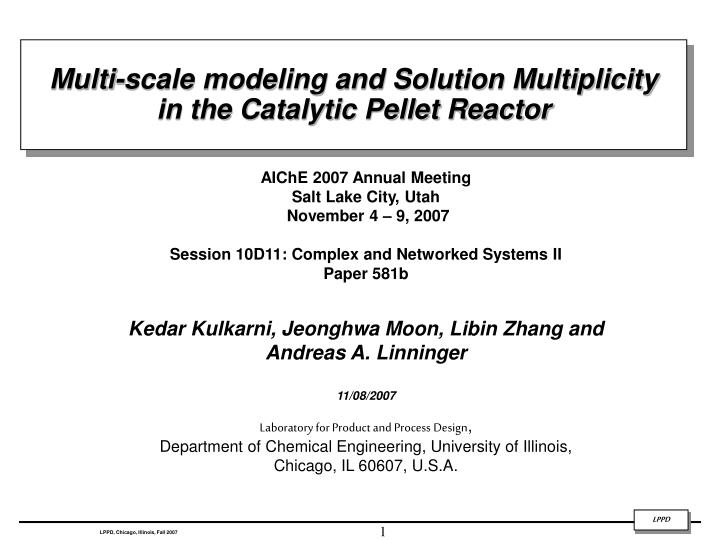
Multi-scale modeling and Solution Multiplicity in the Catalytic Pellet Reactor

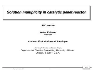
1. Multi-scale modeling and Solution Multiplicity in the Catalytic Pellet Reactor AIChE 2007 Annual Meeting Salt Lake City, Utah November 4 – 9, 2007 Session 10D11: Complex and Networked Systems II Paper 581b Kedar Kulkarni, Jeonghwa Moon, Libin Zhang and Andreas A. Linninger 11/08/2007 Laboratory for Product and Process Design, Department of Chemical Engineering, University of Illinois, Chicago, IL 60607, U.S.A.

2. Motivation: Concentration and Temperature profiles in the reactor depend on which steady states the catalysts are operating in The problem: • Analysis of heterogeneous kinetics in a fixed pellet reactor computationally formidable • Catalysts can operate in different states that correspond to different physically possible overall reaction rates Objectives: • To solve for all physically possible steady states of catalyst pellets for diverse • scenarios • To store and use this information for rapid simulation of the entire reactor

3. Outline • Introduction and overview • Multiplicity in Catalyst pellets • Simultaneous heat and mass transport with reactions in a catalyst pellet - the pellet equations • Methods to solve for ALL pellet profiles: (a) Global bisection method over intervals – Bisection method + ‘shooting’ methods (b) Barrier terrain methods: Global terrain methods + barrier functions (c) Niche evolutionary methods: Niche genetic algorithms + Orthogonal collocation over finite elements • Entire reactor simulation • The whole reactor model – Reaction and transport in Bulk + pellets • Challenges for simulating bulk concentrations and temperatures: (a) Nested collocation approach (b) An multi-scale model based on interpolation • Conclusions and Future work

4. Introduction and overview

5. Cooling Outlet Multi-scale Model B A Tubular Reactor Cooling inlet Packed Catalyst Pellet Bed Catalyst Pellets Micro Pores of Catalysts Introduction and overview Catalytic pellet reactor BULK (MACROSCOPIC) MODEL Mass and energy balances PELLET (MICROSCOPIC) MODEL Coupled mass and energy balance

6. Heat and mass transport in catalyst pelletsSteady state multiplicity in catalyst pellets

7. Reaction and diffusion in catalyst pellets Catalyst pellet Reactant A reacts as it diffuses inside from the catalyst pellet surface Species balance Heat balance Arrhenius reaction rate with Symmetry boundary condition Convective heat and mass transferat the surface

8. Reaction and diffusion in catalyst pellets Under the assumptions of constant pellet properties (heat of the reaction, De and ke) and that the reaction constant ‘k’ is a function of temperature alone we can write: where: where: BC’s:

9. Multiplicity of pellet profiles (Weisz - Hicks): For certain values of γ, β and ϕthere are multiple pellet concentration profiles that satisfy the mass and energy balances and the boundary conditions: For γ = 30, β = 0.6 and ϕ = 0.2 (3 solutions) Our objective is to solve for all possible solutions to the pellet PDE given the constants γ, β and ϕ!

10. Methods to handle catalyst pellet steady state multiplicity Method A: Bisection method over intervals- Based on ‘Shooting’ methods to solve Boundary Value Problems Method B: Barrier terrain methods Method C: Hybrid niche evolutionary methods- Based on Solutions to a system of equations: F(x)=0

11. Method A: Bisection method over intervals – ‘Shooting’ methods Based on “Shooting” methods to solve Boundary Value Problems (BVP) (Weisz and Hicks, 1962; Carnahan et al., 1969) 1 y 2 x BVP x 1 2 x Solution to the BVP obtained with iterative solution of Initial Value Problems (IVP) 1 y IVP 2 x x Solve: x by trial and error

12. The Weisz-Hicks ‘Shooting’ problem We shoot for the Thiele modulus f ! Catalyst pellet equation BVP IVP Set fmodel = x’ (W-H) Solve: Objective: To obtain all possible y0’s that yield

13. BRACKET 1 BRACKET 2 Bisection method over intervals Given the Thiele modulus, f, what is the center concentration (y0)? Equation to solve: Once the correct (y0) is obtained, the pellet profile and the effectiveness factor can be obtained by successive integration of the pellet PDE!

14. Constructing system of equations for Methods B and C Orthogonal collocation over finite elements (OCFE) OCFE Base functions –Lagrange polynomials

15. Constructing system of equations for Methods B and C Pellet BVP Internal nodes (C0) Symmetry BC (C1) Known surface concentration mn equations in mn unknowns!

16. Method B: Barrier terrain methods Global Terrain Method + Barrier functions • Basic concept of Global Terrain Method (Lucia and Feng, 2002) • A method to find all physically meaningful solutions and singular points for a given (non) linear system of equations (F=0) • Based on intelligent movement along the valleys and ridges of the least-squares function of the system (FTF) • The task : tracing out lines that ‘connect’ the stationary points of FTF. • Mathematical background • Valleys and ridges in the terrain of FTF could be represented as the solutions (V) to: V = opt gTg such that FTF = L, for all L єL F: a vector function, g = 2JTF, J: Jacobian matrix, L: the level-set of all contours

17. Method B: Barrier terrain methods Global Terrain Method • Applying KKT conditions to this optimization problem we get the following Eigen value problem Hi : The Hessian for the i th function • Thus solutions or stationary points are obtained as solutions to an eigen-value problem where the Eigen values are identical to the KKT multipliers • Initial movement • It can be calculated from M or H using Lanzcos or some other eigenvalue-eigenvector technique (Sridhar and Lucia, 2001) • Direction • Downhill: Eigendirection of negative Eigenvalue • Uphill: Eigendirection of positive Eigenvalue

18. Method C: Hybrid niche evolutionary methods • Niche methods work on the principles of genetics and natural selection. • They work on a population of possible solutions, while other gradient based methods use a single solution in their iterations. • They are probabilistic (stochastic), not deterministic. • They detect multiple optima sequentially. START Initial population Local optimizer Repair Fitness evaluation Local optimizer Yes Exact solution Convergent? No Natural Selection END Novelty Mating Mutation A) Repair: Individuals are repaired’ using local optimizer for a fixed number of iterations. B) Accelerated solution finding due to local optimizer: When the population is ‘dense’ enough about a solution, we use the local optimizer to find solution.

19. Niche Evolutionary Methods • Genetic algorithms for problem with multiple extrema (multi-modal) • Use the concept of fitness sharing • Restricts the number of individuals within a given niche by “sharing” their fitness, so as to allocate individuals to niches in proportion to the niche fitness niche radius No fitness sharing Fitness sharing

20. Example: Himmelblau’s function individuals Initial guess solution Maxima (3.58,-1.86), (3.0,2.0), (-2.815,3.125), (-3.78,-3.28)

21. Shooting + Bisection (A) OCFE + Hybrid niche (C) Results using methods A and C γ = 30, β = 0.3, ϕ = 0.5 γ = 20, β = 0.8, ϕ = 0.2 Dimensionless pellet concentration (y) vs. Dimensionless pellet radius (x): γ = 30, β = 0.6, ϕ = 0.1 γ = 40, β = 0.3, ϕ = 0.3

22. Comparison of methods A and C All results on a Pentium IV machine (2.53 GHz, 1 GB RAM)

23. Comparison of methods A and C Comments: • Shooting + Bisection (method A) is an approach to solve Boundary value problems in particular. • OCFE + Hybrid Niche (method C) is a general approach to identify multiple solutions to an equation system. OCFE + Hybrid Niche (method C) Shooting + Bisection (method A) Advantages: • Does not need initial guesses • Does not need gradient information Disadvantages: • Works only if the solution exists in the intervals considered Advantages: • Does not need initial guesses • Does not need gradient information Disadvantages: • The finite element grid should have the configuration to get a valid solution

24. MULTI SCALE MODELING

25. Whole reactor simulation model Species transport BULK (MACRO) MODEL Heat balance Reactor BC’s Arrhenius reaction rate where Reaction and diffusion in pellets PELLET (MICRO) MODEL Pellet BC’s Effectiveness factor

26. N n e w P E W s S Whole reactor simulation model – Finite volume methods Reactor domain divided into small finite volumes Integrate transport equations over finite volumes Nonlinear algebraic equations

27. Whole reactor simulation model – challenges 1) No analytical solution possible 2) The effectiveness factor h is an implicit function of the bulk C and T Bulk equations: When we solve for the bulk C and T iteratively, the pellet PDE has to be solved at each iteration, to obtain the h! 3) Use of shooting + bisection (method A) or OCFE + Hybrid niche (method C) at each iteration will lead to large computational times.

28. Method I: Direct iterative simulation with nested collocation Given parameters: E, kref, DA, Kb, De, ke, DH NESTED LOOP FOR h Initialize: (a) Bulk C0 and T0 profile (b) Pellet profile (y0) and effectiveness factor h0 Obtain Bulk Ck1 and Tk1 profile Calculate: g(Ck1,Tk1), b(Ck1,Tk1), f(Ck1,Tk1) Obtain Pellet yk2 and hk2 Quasi-Newton update: Pellet yk2 +1 and hk2 +1 k1=k1 +1 k2=k2 +1 Residual < e NO YES Quasi-Newton update: Bulk Ck1 +1 and Tk1 +1 profile Residual < e NO YES DISPLAY SOLUTION:Bulk C* and T* profile

29. Interpolation based multi scale model Disadvantages of the nested collocation model • Initial guess dependence of the nested loop for the effectiveness factor, h. • Computation of the pellet profile inevitable, when all you need is the effectiveness factor, h. New interpolation based multi scale model • Prepare a map: • Since h is parametrized in three dimensionless quantities g, b and f, we interpolate in this space to obtain the h for the given gk, bkand fk at the k-th iteration.

30. Method II: Interpolation based multiscale model Given parameters: E, kref, DA, Kb, De, ke, DH REPLACES NESTED LOOP FOR h Initialize: (a) Bulk C0 and T0 profile (b) Pellet profile (y0) and effectiveness factor h0 Obtain Bulk Ck1 and Tk1 profile Calculate: g(Ck1,Tk1), b(Ck1,Tk1), f(Ck1,Tk1) Interpolate in the g, b, f space to obtain h k1=k1 +1 Quasi-Newton update: Bulk Ck1 +1 and Tk1 +1 profile Residual < e NO YES DISPLAY SOLUTION:Bulk C* and T* profile

31. Interpolation based multi scale model Effectiveness factor map INPUT:g, b and f OUTPUT:h

32. Results using the two methods Dimensionless Cbulk and Tbulk vs. the length of the reactor

33. Comparison of the two methods

34. Comparison of the two methods The use of 3D interpolation is preferable over nested collocation because: • It eliminates the convergence failure problems associated with using nested collocation • It eliminates the need to solve for pellet profiles that is inevitable with nested collocation • The simulated bulk concentrations and temperatures are obtained about 5 times faster with an insignificant loss of accuracy

35. Conclusions and future work Catalyst pellets • Discussed three methods to handle steady state multiplicity in catalyst pellets: Method A: Shooting + bisection method Method B: OCFE + Hybrid Niche methods Method C: Barrier terrain methods Simulating the entire reactor • Challenges for simulation – heterogeneous reaction with transport in the reactor while accounting for pellet reaction/transport • Proposed a multi-scale interpolation approach that saves computational cost significantly Future work • Multiple bulk concentration and temperature profiles corresponding to multiple pellet states • Inversion multiplicity due to catalyst pellet steady state multiplicity

36. Thank you!

37. Formulating the ‘shooting’ problem Catalyst pellet equation BVP IVP

38. R R’=aR Explanation Enforce the co-ordinate transformation on x in (A): (BVP) (IVP) Now If we integrate (IVP) until: For the BVP: Thus: and