Download
1 / 15
150 likes | 247 Views
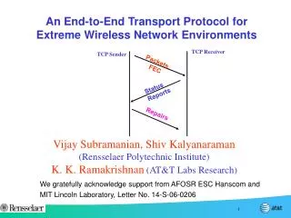
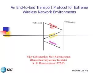
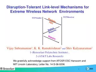
Robust and Loss-Tolerant Link and Transport Protocols for Wireless Network Environments. Vijay Subramanian + , Shiv Kalyanaraman + , K. K. Ramakrishnan * + (Rensselaer Polytechnic Institute) * (AT&T). Motivation.

E N D
Robust and Loss-Tolerant Link and Transport Protocols for WirelessNetwork Environments Vijay Subramanian+, Shiv Kalyanaraman+, K. K. Ramakrishnan* +(Rensselaer Polytechnic Institute) *(AT&T)
Motivation • Explosion in the deployment of wireless links implies that performance over multi-hop wireless links is important. • It is also desirable that link-level latencies are kept small and bounded. (VoIP traffic, streaming media) • End-end loss rates may be significantly higher than what can be tackled by state-of-the-art TCP variants (TCP-SACK) (5% packet error rate) • Our objective is to • Design a link-level protocol that can provide small residual loss rate with small delays • Design a transport-protocol that can tackle high end-end loss rate (0-50%) while providing high goodput.
Motivation: TCP-SACK under Lossy Conditions • Exponential falloff in performance with PER • Performance VERY bad for the combination: • 5%+ PER • 100 ms+ RTT
Design Objectives • Link layer should export as low a residual loss rate to the upper (transport) layer as possible. • Need not be 0 however. Link should make a best-effort while not over-protecting. • Link-layer latency/delay should be as small as possible. • Unlimited ARQ attempts will lead to variable and large latencies which is not suited for VOIP-like traffic. • This implies that the number of ARQ attempts should be limited and small. • Link-layer protocol needs to operate on small timescales. • Disruption / Error period can be smaller or larger relative to the link RTT. • Link- protocol should be robust under such scenarios. • At the transport layer, reliability is needed. • Residual loss rate should be nil. • Time scales of operation are large. • The end-end path may span multiple hops and the feedback may take time to reach the sender.z
Common Building Blocks… • Loss Estimation: • The sender estimates link-level Packet Error Rate (PER) on the lossy link for the LL protocol. • At the TCP level, the sender estimates the PER on an end-to-end basis over the entire path. • Fragmentation/Segmentation • At the transport layer, a window is granulated to contain a minimum number of TCP segments (avoid timeouts and generate acks/dupacks) • At the link layer, a packet is split into a number of fragments to achieve a similar effect. • Proactive FEC • PFEC is set in the initial transmission and can be seen as insuranceagainst anticipated loss (calculated based on estimated loss rate.) • Reactive FEC: • If PFEC is insufficient to recover the data, retransmission consisting of RFEC is used to reach the required number of packets/fragments.
Building Blocks… • ECN-Environment (TCP-only): • We infer congestion solely based on ECN markings. • Window is cut in response to • ECN signals: hosts/routers have to be ECN-capable. • Timeouts: The response to a timeout is the same as with standard TCP. • Window Granulation and Adaptive MSS: • We ensure that the window always has at least G segments ( allows for dupacks to help recover from loss at small windows) • Avoids timeouts • Window size in bytes initially is the same as normal SACK TCP. • Initial segment size is small to accommodate G segments. • Packet size is continually adjusted so that we have at least G segments. Once we have G segments, packet size increases with window size. • Loss Estimation: • The receiver continually tracks the loss rate and provides a running estimate of perceived loss back to the TCP sender through ACKs. • We use anEWMA smoothed estimate of packet erasure rate
Building Blocks … • Proactive FEC: • TCP sender sends data in blocks where the block contains K data segments and R FEC packets. The amount of FEC protection (R) is determined by the current loss estimate. • Proactive FEC based upon estimate of per-window loss rate (Adaptive) • Reactive FEC: • Upon receipt of a dupack atTCP, Reactive FEC packets are scheduled based on the following criteria. • Number of Proactive FEC packets already sent. • Cumulative hole size seen in the decoding block at the receiver. • Loss rate currently estimated. • Reactive FEC to complement retransmissions • both used to reconstruct packets at receiver • DATA, PFEC and RFEC follow the spirit of TCP semantics (self-clocking and packet-conservation principle.)
Binomials for different loss rates, N =20 • As Npq >> 1, better approximated by normal distribution (esp) near the mean: • symmetric, sharp peak at mean, exponential-square (e-x^2) decay of tails (pmf concentrated near mean) 10% PER 30% PER Npq = 4.2 Npq = 1.8 N = 20 for all cases 50% PER Npq = 5
FEC implications • By setting PFEC ratio = , we ensure that more than half the blocks are recovered in one round. • Since the distribution is peaked, the PFEC wastage is less than a uniform distribution (most blocks waste only 1 or 2 PFEC units) • Setting PFEC ratio significantly lower than => PFEC waste low, but will move most of recovery burden to future rounds. • The effective “N” used for RFEC can be very small for any “efficient” RFEC strategy, and hence RFEC phase is more fragile (i.e. all RFECs can be lost with higher probability).
Round 2 Issues • Residual distribution: “chopped binomial” ! • Peak in original binomial distribution • Pfec “chops off” the binomial distribution • Pfec ratio of + => chops upto the mean, and one beyond that • Pfec ratio of - => chops binomial upto - • Residual distribution of required units (X) in round 2 looks like a chopped binomial. • For pfec ratio > , this has a peak at X = 1, and decays very fast (e-x^2) • Small N problem in Round 2: • The frequency-weighted average of X is very small (due to peak at X =1 and fast decay beyond). • Even if X is scaled up based upon the loss rate (i.e. by 1/(1-p) ) to get N = Y, this Y value will be small for p < 50% for small values of X. • Binomial distribution with small N => high probability of all units lost in round 2. • Necessary to overprovision RFEC beyond just a scaling by loss rate. • Need to add several standard deviations to ensure a minimum N to reduce the all-unit-loss probability.
Wasted RFEC units (480, 240, 96, 30…) • out of (1108, 628, 280, 97…) RFECs sent. • * Total RFEC sent: 2145 • * Total wasted RFEC: 855 {39.8% of 2145} • Total units sent (including round 1): 22145 • RFEC waste/Total: 3.86% vs • PFEC waste/Total: 10% 3.6:1 15:1 ratio! Y = 15 RFEC Issues & Effects Total RFEC in Round2 (Y) = (X + 3)/(1-p) Add 3 and scale up by (1-p), and round-off to nearest integer
Bottom-Line Numbers & Simulation Validation Analysis Numbers: (p = 50%) Goodput = 3.61 Mbps vs 5 Mbps (max) PFEC waste: 1.0 Mbps = 10% RFEC waste: 0.39 Mbps = 3.9% Residual Loss : 0.0% Weighted Avg # Rounds: 1.13 LL-HARQ Simulation Numbers: Goodput = 3.59 Mbps vs 5 Mbps (max) PFEC waste: 0.998 Mbps = 9.97% RFEC waste: 0.39 Mbps = 3.94% Residual Loss : 0.034% Weighted Avg # Rounds: 1.12 Analysis Numbers: (p = 10%) Goodput = 8.15 Mbps vs 9 Mbps (max) PFEC waste: 0.57 Mbps = 5.7% RFEC waste: 0.28 Mbps = 2.78% Residual Loss : 0.53% Weighted Avg # Rounds: 1.11 SimulationNumbers: (p = 10%) Goodput = 8.08 Mbps vs 9 Mbps (max) PFEC waste: 0.59 Mbps = 5.9% RFEC waste: 0.26 Mbps = 2.6% Residual Loss : 0.0% Weighted Avg # Rounds: 1.11
Bursty Case Comparison Analysis Numbers: (p = 25-75%) Goodput = 2.88 Mbps vs 5 Mbps (max) PFEC waste: 1.13 Mbps RFEC waste: 0.994 Mbps Residual Loss : 4.2% Weighted Avg # Rounds: 1.90 Simulation Numbers: (p = 25-75%) Goodput = 2.74 Mbps vs 5 Mbps (max) PFEC waste: 1.47 Mbps RFEC waste: 0.662 Mbps Residual Loss : 4.02% Weighted Avg # Rounds: 1.27